Introduction

The humanity is now going through the post-industrial stage of technological development. The post–industrial economy implies radical transformations not only of manufacturing but also of extracting industries. In all likelihood, the disparities between economic sectors regarding the degree of processing, automation and staff qualification levels will continue to grow. Tax regulation tools that are currently applied will be still in use although it seems quite possible that the degree of differentiation in this sphere will also increase.

To predict the future of tax regulation, it is necessary to consider how sensitive are different sectors to the current level of tax burden. Our main hypothesis is that industries with higher degrees of processing and, consequently, higher levels of technological intensity and complexity of production are more sensitive to taxation. Therefore, extractive industries, which rely on exploitation of natural resources and rental income, should be much less susceptible to tax. Thus, the purpose of this study is to model the relationship between production in different sectors of the Russian economy and taxation. To this end, we are going to build econometric dependencies of production growth on tax burden in the 2000s and 2010s.

Tax burden and production growth: literature review

It is generally accepted that that potential economic growth of different countries is to a significant extent determined by their financial resources [1]. Since governments raise financial resources through taxes, increasing tax revenue contributes to the general prosperity of society and to economic growth.

However, the influence of taxes on economic activity is far from being simple or straightforward. Some studies show that this influence is generally positive [2, 3] while others demonstrate a negative relationship between economic growth and the increasing tax burden [4]. This is no surprise since taxes can have two opposite effects: on the one hand, they can stimulate economic activity by increasing state revenue and investment and, on the other, taxes can have an adverse impact on economic activity if the tax burden proves to be excessive.

Originally, the idea that there is a certain level of tax rates beyond which taxes will stifle economic growth instead of spurring it appeared in the US. This idea belonged to Arthur Laffer, who proposed his famous 'Laffer curve'. This term was coined by Laffer's friend American economist and journalist Jude Wanniski. In his article Wanniski told the story of a fabled restaurant dinner where Laffer drew the dependency of tax revenue and tax rate on a napkin [5]. Laffer himself later elaborated this theory in a series of works [6, 7, 8].

Laffer's concept was widely discussed in research literature. Canto et al. [9] were among the first who used the Laffer curve to calculate the tax rate that would maximize tax revenue. Afterwards, this methodology was often used to estimate the impact of tax burden on tax revenue and economic growth. There were also studies that tested its applicability in other areas, for instance, in relation to countries' debt [10] or in the conditions of post–Communist transformations of economy [11]. Stuart used the Laffer curve to calculate that the optimal marginal tax rate on labour income for the 'representative' Swede was at the level of 70%. In reality, the effective marginal tax rate grew from 50% in 1959 to 80% in the early 1980s, which explains up to 75% of the decline in the growth rate of the Swedish GNP [12]. The average effective tax rate, maximizing the volume of output, for Sweden in 1979 was computed to be 54–62% of total national income [13]. In the Netherlands, the marginal income tax rate was 70% in 1985 while its actual value was nearing the limits and was at the level of 67% [14].

The optimal marginal tax rate, maximizing tax revenue, for twelve OECD countries in 1996 varied between 53 and 60% of GDP [15]. For the US, Strulik and Trimborn [16] found a very flat Laffer curve for all capital taxes and calculated that total tax revenue could increase by about 0.3–1.2% after abolishment of the tax on capital gains. Laffer curves for the US, the EU–14 and individual European countries have shown that tax burden does not peak and can be increased in the US by 30% with labor taxes and 6% with capital taxes. For the EU–14 these figures are 8% and 1% respectively [17]. Tax burden in China has not reached its optimal level so far, which, according to Lin and Jia, is 40% of GDP [18]. Analysis of the Ukrainian economy in 1996–2011 has shown that the optimum point for economic growth was 38.2% [19]. Similar calculations have been carried out for the Russian economy in 1989–2000 and showed the optimal tax burden at the level of 36.5% [20].

Some economists criticized the Laffer theory for the lack of empirical evidence to support it [21; 22]. In a general equilibrium model, some properties of the Laffer curve do not necessarily hold [23]. Moreover, results of the Laffer curve may be unreliable for the labor supply elasticity [24]. Doubts were voiced about the very existence of the optimal tax rate and the possibility of calculating it [25].

Opposed to this skeptical view is the view shared by many Russian, Ukrainian and Georgian economists (Y. Ananiashvili, E. Balatsky, B. Bukach, V. Vishnevsky, A. Gusev, M. Kakaulina, G. Loladze, S. Londar, I. Mayburov, T. Merkulova, S. Movshovich, V. Papava, A. Sokolovskaya, L. Sokolovsky, S. Chugunov and others). They believe that the Laffer curve can be a useful tool of analysis. Gusakov, Zhak and Balatsky introduced the notion of the Laffer points of the first and second kind with the corresponding production and fiscal curves [20, 26]. Such modification of the Laffer theory implies two levels of analysis and two dependencies. This, in turn, has led Mayburov and Sokolovskaya to propose the notions 'area of fiscal controversies' and 'additional tax trap' [27]. Georgian and Ukrainian economists have made a considerable contribution to the methodology of computing Laffer points [28, 29]; analysis of the impact of tax burden on technology of production and amount of resources used [30] and aggregate demand [31]. They also worked to improve the methodology of calculating effective tax rates [32].

The graphic visualization of the production and fiscal curves has been demonstrated to change depending on the initial assumptions [33]; on such factors as the shadow economy [34], people's preferences [35], mechanisms of resource use to balance the budget [36], the macro–economic situation in the country [37], and tax 'migration' [38]; and on the choice of a specific tax [39; 40]. Ananiashvili and Papava propose an approach based on Laffer–Keynesian synthesis, but so far this idea has made little progress [29].

Even though there is a vast body of research on the relationship between tax burden and economic growth, it should be noted that such estimates are usually rather general and do not take into account the specifics of regions or economic sectors, which limits the practical applicability of these results. Sensitivity of sectors and regions to tax burden can be affected by various factors and differ severalfold. In recent years, among Russian economists, there has been a surge of interest in the effects of tax burden, especially regarding specific sectors of economy and regions.

For example, Kakaulina calculated the critical values of the optimal tax burden in regions with different resource potential [41]. In another study, she identified the general quantitative patterns in the way tax burden influences economic growth in regions with different industrial profiles and calculated the optimal tax burden for these regions [42]. Her calculations have shown that for Russian regions specializing in retail trade (e.g. Moscow region), the values of the 'area of fiscal controversies' (difference between the values of Laffer points of the first and second kind) are considerably higher than for regions specializing in agriculture (Krasnodar region), mining and metallurgy (Sverdlovsk region), education and R&D (Novosibirsk region): 22.1–34.9% against 15.6–21.2%,17.5–20.5%, 18.9–22.6% respectively [42].

Other studies in this field revealed a number of drawbacks of the Russian tax regulation system and led the researchers to formulate recommendations on how it can be improved. For example, it was shown that the differences between the Russian and international methods of calculating the tax burden for specific sectors result in underestimation of the effective tax burden in Russia [43]. Moreover, tax burden is distributed unevenly across sectors: it is higher in the manufacturing sector, which means that it is necessary to incentivize innovation in manufacturing enterprises, for example, through differentiated corporate tax rates [44]. Kakaulina analyzes the tax burden for types of economic activity in 2009–2017, measured as the ratio of the sum of tax payments (free of personal income tax) and social security contributions to net value added of enterpises involved in a certain type of economic activity [45]. She also points out the fact that the heaviest tax burden is borne by extractive and manufacturing industries and describes a general methodological approach to calculation of tax burden that would ensure accuracy and comparability of results [45].

 Our article continues this line of research and seeks to improve the instruments that can be used to estimate economic sectors’ sensitivity to tax burden.

Methodology

To build econometric dependencies, we are going to use a traditional method based on revealing the connection between the volume of output generated by industrial sectors and tax burden understood here as the share of total turnover in an industry collected in different forms of tax and constituting tax revenue to the country's consolidated budget. We use as a point of departure the assumption that the taxes paid by enterprises are of equal status and, therefore, it does not matter which specific tax rates rise or fall. What matters is the amount of revenue that the producer is left with after all the obligatory payments have been made.

As mentioned earlier, such analysis is commonly referred to in research literature as 'Laffer’s analysis'. This approach usually implies that we need to build a non–linear production curve dependent on the average tax burden and a fiscal curve, which is the dependency of tax revenue on the average tax burden multiplied by the production output (taxable base). Although this approach has been productively applied in some studies, it has not been widely used to date.

Balatsky and Ekimova attempted to apply Laffer's approach a bit differently and built econometric dependencies of production growth rates and the average tax burden [46]. This is a dynamic dependency since the production growth rate in perсentage points is in the left–hand side of the equation and the tax burden in percentage points is in the right–hand side. In a traditional static dependency, production growth in the left–hand side is given in absolute cost values while in the right–hand side, labour productivity is expressed in absolute natural values; capital, in absolute cost values; and tax burden, in relative values (percentage points). Although this approach holds some promise, in its original version it is not without certain faults and is suitable only for a first experiment in a series of such analytical computations. The drawbacks that need to be addressed are as follows.

First, no control variables were used in models, which means that the dynamics of production could not be considered separately from the general trend. Second, the authors used a quadratic dependency on tax burden, which, strictly speaking, is not correct since explanatory variables should not be multicollinear while it was initially known that in the resulting models they would be functionally (!) connected. Third, to evaluate the econometric dependency, the intercept term was nullified, which shifted the estimates and lead to less accurate and reliable results.

Our study seeks to remedy these drawbacks. The peculiarity of the procedure we are going to apply is that we are going to construct an explanatory variable in the form of an a priori non–linear fiscal aggregate with a predetermined parameter. After conducting a series of computational experiments, we expect to find significant econometric dependencies by increasing the value of the parameter in the fiscal aggregate. This procedure will allow us, on the one hand, to avoid multicollinearity of explanatory values and, on the other, to keep the initial assumption that there is a non-linear relationship between production and tax burden.

Thus, through the resulting models we will discover parabolic and quasi–parabolic dependencies and will be able to apply Laffer's analysis to identify the most significant – optimal and critical – points of tax burden. These points can be used as a kind of markers for tax regulation and prediction of industries’ responses to changes in their tax burden.

Fiscal profile of the Russian economy as a whole

To shed light on the general situation in the Russian economy, we are going to build a model of the dependency between GDP growth rates and tax burden q=T/Y, where Y is GDP in current prices and T is tax revenue in current prices. In this case, parameter q characterizes tax burden borne by producers as a share of GDP.

In this section, we will consider the period from 1996 to 2019. The statistical input data were provided by the official reports of Rosstat and the Federal Tax Service (FTS) (Table 1). For other models we used the same sources of statistical data but the period was different.

Table 1

Input data for model (1) for the Russian economy as a whole

We use GDP growth rates (I) as an output variable and employment growth rates (J) as a control variable. With the help of this variable, we can 'neutralize' the general trend of expanding/shrinking economy and use the fiscal aggregate as an instrument for adjustment of the regulation regime. As we mentioned above, our intention is to build a certain a priori non–linear fiscal aggregate, which is going to serve as one variable in an econometric dependency. This will allow us to test the hypothesis about the non–linear impact of tax burden on production. In relation to the Russian economy, this fiscal aggregate takes the form of a quadratic function, which looks the following way: W=(q–kq²), where k>0 is the coefficient that takes different values in the process of building the econometric dependency. This approach enables us to conduct many computational experiments with different k values. The resulting model based on the data shown in Table 1 looks the following way:

            (1)

N=24; R²=0,46; DW=1,88; E=2,61%,

where N is the number of observations; R², the determination coefficient; DW, the Durbin Watson statistic; E, the average approximation average (in %); and t–statistics are given in parentheses for all regression coefficients. The resulting model satisfies the main statistical tests and has a high approximation accuracy; the fiscal aggregate is significant at the level of 10%.

Thus, there is a parabolic dependency between economic growth and tax burden, which confirms the classical hypothesis about the non–linear impact of taxes on production activity.

If we take InJ as the average value in the whole observation period, then lnJ=4,61. Then, as the calculations show, the optimum tax burden point is q*=38,5%; if InJ is taken for each year, then point q* will float in time, which is why, for the sake of simplicity, we are going to use average values. The optimum point corresponds to the economic growth index I*=105,4%. Thus, provided that the tax system is perfectly adjusted, the yearly GDP growth in Russia will be 5.4%.

Special attention should be given to those two points of the tax burden where GDP growth index is 100%, which corresponds to the simple reproduction mode. We need fairly straightforward calculations to show that this value can be reached if the tax burden is q₀=7,7% and q₀₀=69,2%. This is an optimistic result, since the upper limit beyond which the national economy will plunge into recession is quite far from the effective tax burden. We may even say that the value of the upper limit q₀₀ is unrealistic. Furthermore, the effective tax burden is significantly below the optimum point q*=38,5%, that is, the Russian economy is on the rising arc of the parabolic curve (Fig.1).

Fig.1. Geometrical interpretation of function (1) for the Russian economy as a whole

Model (1) shows that the Russian economy as a whole has low sensitivity to tax burden while the current figures do not give us any indication of excessive tax burden on Russian enterprises. We are going to return to this paradoxical fact in the final section of our paper.

Fiscal profile of the manufacturing sector

As is often the case, the situation in the economy as a whole can be quite different from the situation in individual sectors. Therefore, in the following sections we are going to look at how different sectors respond to taxation tools.

Table 2

Input data for model (2) for the manufacturing industry

First, let us concentrate on the manufacturing industry. Unlike the previous case, this time the fiscal aggregate takes the form of the following functional dependency: W=[q–k*ln(q)], where k>0, as before, is a varying coefficient. Like in model (1), in equation (2), employment in the sector is a control variable and there is dummy variable F, which takes value F=1 for 2009 and 2015 and F=0 for the other years. This dummy variable is also used as a control variable to distinguish between growth phases (F=0 if I>100%) and decline phases (F=1 if I<100%) in production. Variable I corresponds to turnover growth in the manufacturing sector. We should put particular emphasis on this fact because in model (1) we used a ‘cleaned’ indicator of domestic production – GDP. Moreover, we have an extremely short time series (2006–2007), due to the lack of data for other years because the web–site of the FTS provides sector–specific information only starting from 2006. The resulting model based on the data shown in Table 2 looks the following way:

    (2)

N=14; R²=0.79; DW=1.91; E=2.04%.

Model (2) was found to be satisfactory and can be used for analytical calculations. Function (2) is a quasi–parabolic dependency with a maximum point, which corresponds to I*=107.1% with tax burden q*=5.7% (like before, we are going to use the average value for the whole period lnJ=4.60). Thus, provided that the tax system is perfectly adjusted, the potential yearly production growth in the manufacturing industry will be quite substantial – over 7%.

 For model (2), the critical points where the production growth rate is 100% take the following values: q₀=3,5% and q₀₀=8,7% and we take into account the growth phase (F=0). The decline phase (F=1) is described by a similar curve, though shifted slightly downwards. This fact signifies that when the industry is in the decline phase, it is less sensitive to tax regulation. For instance, even when the tax burden is optimal (5.7%), the production rate is only 93.0%, that is, tax regulation alone is unable to pull the industry out of its slump and there is a need for other factors and stimuli.

 In its growth phase, the manufacturing industry demonstrates a higher sensitivity to tax burden, which can be explained by the fact that the effective tax burden in the given period varied between 6.0 and 8.6%. This leads us to at least two important conclusions: first, the Russian manufacturing sector is on the descending branch of the non–linear production dependency (2) (q*=5,7%<q=6,0–8,6%) (Fig. 2). Therefore, such tax regime slows down the growth in the sector and even at this moment impedes it from realizing its production potential. Second, in some years the effective tax burden came close to the right critical point (q=6,0–8,6%<q₀₀=8,7%). In this case, a more rigorous tax regime for this sector may provoke a slump in production. In other words, by setting the tax burden at its current level, fiscal policy–makers are walking a fine line since tax regulation is now quite close to triggering a full–blown recession.

Fig.2 Geometrical interpretation of function (2) for manufacturing

Thus, our calculations have brought to light an interesting asymmetry in the manufacturing industry's response to the tax burden: in its growth phase, the sector appears to be highly sensitive to taxation while in the recession phase, the taxes lose their stimulting effect.

Fiscal profile of the extractive industry

As it will be clear from our subsequent calculations, specific characteristics of economic sectors determine the degree of their sensitivity to tax burden. This is particularly evident in the extractive industry. Like in the preceding model (2), variable I reflects gross revenue growth in the sector. We use employment growth as a control variable and introduce dummy variable F, which takes value F=1 in 2008 and 2014, which were officially recognized as recessive years, for other years the variable takes value F=0.

Table 3

Input data for model (3) for the extractive industry

Our computational experiments based on the data from Table 3 have resulted in the following econometric dependency for the extractive industry:

      (3)

N=14; R²=0.61; DW=2.45; LM1=1.24; KM2=1.35; LM3=2.35; E=0,80%.

 In model (3), the results of the Durbin–Watson (DW) test were inconclusive as the DW statistic fell within an uncertainty area, which is why we additionally used the Breusch–Godfrey serial correlation LM test. It showed that in model (3) there are no first–, second– or third–order autocorrelations. Model (3) satisfies all the diagnostic tests. Function (3) is completely the same as function (2): it is a convex dependency with the maximum point I*=103.1% and the optimal tax burden q*=40.9% (as before, for simplicity we take the average of InJ for the whole period: lnJ=4.61) (Fig. 3). For model (3), the critical points where the production growth index is 100% for the growth phase (F=0) take the following values: q₀=27.5% and q₀₀=58.2%.

Fig.3 Geometrical interpretation of function (3) for the extractive industry

If we compare the models for the manufacturing and extractive industries, we can see a whole range of differences between them.

First, the factor of employment in the extractive industry has a negative value, which contradicts the classical premises of production functions. This paradox can be explained the following way: the extractive industry's performance is determined by global oil prices and oil demand rather than by its human capacity. In other words, the number of employees in this industry depends on the level of oil production. If the market conditions are adverse, workers retain their jobs but turn into a dead weight for their enterprises, which is what signifies the negative value of the coefficient in model (3) with the logarithm of the employment index. Apparently, the use of rotation shiftwork cannot fully resolve this issue. It is also possible that an increase in labour productivity and modernization in the sector contribute to the paradox described above.

Second, for the extractive industry, the width of the corridor of the tax burden values, within which the industry does not risk slipping into recession, far exceeds the similar figure for the manufacturing industry: 27.5–58.2% against 3.5–8.7%. In other words, the areas of a relatively safe variability of the tax burden for the extractive industry is 30.7 percentage points while for the manufacturing industry it is 5.2 percentage points, that is, we are dealing with an almost 6 times difference. Thus, the manufacturing industry’s sensitivity to tax regulation is considerably higher than that of the extractive industry.

Third, the effective average yearly tax burden on the extractive industry was 36.3%, while the optimum tax point, q*=40,7%. The effective tax payments exceeded the optimum point only in 2006, 2008, 2014 and 2018. Therefore, most years the extractive industry was on the rising arc of curve (3) and never closely approached the right critical boundary.

Fourth, there is a huge difference between the tax burden on the extractive and manufacturing industries. While the average tax burden of the former is 36.3%, for the latter this figure is 6.9%, that is, the difference can be up to 5.3 times. This may seem strange but in fact it is quite natural if we take into consideration the technological characteristics of each sector. The fact is that the extractive industry uses raw materials at a minimum extent and benefits from the natural resource rent while intermediary consumption (raw materials, semi–finished goods, etc) makes up a considerable proportion of the prices in the manufacturing industry. Moreover, unlike the manufacturing industry, the extractive industry is dominated by natural monopolies. Hence, the extractive industry occupies a privileged position, which is why it can bear a heavier tax burden.

Our calculations have shown that applying the same tax policy in different sectors is not the optimal solution because it does not take into consideration their technological characteristics and market positions.

Fiscal profile of manufacture of coke and petroleum products

Let us now go back to manufacturing and focus on such 'intermediate' sector as manufacture of coke and petroleum products. The methodology and statistical base remain the same. As in previous cases, variable I demonstrates gross revenue growth and variable G, price growth on the global oil market (prices are given in dollars) (control variable). The result of our computational experiments based on the data from Table 4 is the following econometric dependency, which is similar in structure to the two previous ones:

                   (4)

N=14; R²=0.54; DW=2.08; E=2.43%.

Table 4

Input data for model (4) for manufacture of coke and petroleum products

Model (4) satisfies all the statistical tests. Function (4), like previous dependencies, is quasi–parabolic with a maximum point that takes the value I*=104.7% with the optimal tax burden q*=2.9% (we take the average value of InG: lnG=4.62). For model (4), the critical points where the productions growth index is 100% take the following values: q₀=0.8% and q₀₀=7.5% (Fig. 4).

Fig.4 Geometrical interpretation of function (4) for manufacture of coke and refined petroleum products

Importantly, to build model (4), we didn't have to use a dummy variable, which shows that this sector is relatively recession–proof and that the role of the control variable is played by the oil price indices. The employment index of the sector was insignificant in all combinations. Apparently, the sector is more dependent on global oil prices than the size of the workforce.

Our calculations show that the average tax burden throughout the whole period was 5.7%, which is slightly above the optimum point q*=2.9%. Thus, the sector was on the descending arc of the non–linear dependency on tax burden. At the same time the effective tax burden never exceeded the right critical point (q<q₀₀=7.5%), although in 2011 and 2012 it came close to this point.

 Thus, the situation in the sector is quite similar to that of the whole extractive industry. The difference is only that for the oil processing sector the optimum point is much lower: q*=2.9% against q*=5.7%. Therefore, manufacture of coke and petroleum products is even more sensitive to taxation than the manufacturing industry and, consequently, even more sensitive to this type of regulation.

Fiscal profile of the chemical industry

Let us now look at the sector with more extensive processing – the chemical industry. The methodology and statistical base remain the same. Variable I shows the sector's gross revenue growth and variable P, labour productivity growth (control variable). Dummy variable F takes value F=1 for 2009 and 2014 and F=0 for the other years. The result of our computational experiments based on the data from Table 5 is the following econometric dependency, which is quite similar in structure to the previous models but is a little more complex for the control variable:

  (5)

N=14; R²=0.80; DW=1.93; E=1.59%.

Table 5

Input data for model (5) for the chemical industry

Model (5) satisfied all the statistical tests and is suitable for further analysis. Like the previous models, dependency (5) is quasi–parabolic with I*=106.5% as the maximum point, with the optimal tax burden q*=2.6% (average value P=105,8). For model (5), the critical points, where the production increase index is 100%, take values q₀=1.4% and q₀₀=4.4% (Fig. 5).

Fig.5 Geometrical interpretatation of function (5) for the chemical industry

Our analysis shows that for five years the sector was on the left (rising) arc of function (5) and for nine years, on the right (downward) arc. In general, the average effective tax burden q=2.8% was below the optimum point q*=2.6%.

What distinguishes the model built for the chemical industry is that it has an extremely narrow corridor of acceptable tax burden values ∆q=q₀₀–q₀, which is only 3.0 percentage points and is the record low among the other sectors in question (Table 7). This signifies that the chemical industry is highly sensitive to fiscal regulation and, therefore, requires a specially tailored approach.

Yet another peculiarity of model (5) is a convex quasi–parabolic dependency of the sector's turnover growth on labour productivity growth. For the average tax burden in the whole period q=2,8%, the optimal level of labour productivity growth is 101.5%, with the production growth rate of 103.1%. Thus, here we are dealing with an interesting effect: modernization in the industry should be thoughtfully and carefully dosed, otherwise, its production growth will decline. The lack of data prevents us from offering a more detailed explanation to this phenomenon. We can suppose, however, that the chemical industry is quite sensitive to any modernization attempts, to which it may react by reducing output. There is logic in this since any serious modernization implies that the enterprise will have to pause its production (or a part of it) in order to change, modify or re–engineer equipment and thus possibly fall behind its production schedule.

In sum, to avoid reduced production in the chemical industry, which is one of the country’s most efficient sectors, a carefully adjusted tax policy is necessary, which also applies to technological innovation in the industry. All of the above shows that there are natural limits to the speed of the sector's development.

Fiscal profile of electrical engineering

At the next stage of our analysis we are going to consider the sector in the avant–garde of technological progress – electrical engineering. The methodology and statistical base remain unchanged. Variable I corresponds to gross revenue growth in the sector and variable P, to labour productivity growth (control variable). This time the fiscal aggregate includes a control variable: W=[lnP–(q–k*ln(q))]. The result of our computational experiments based on the data from Table 6 is the following model:

                       (6)

N=14; R²=0.77; DW=1.95; E=4.73%.

Table 6

Input data for model (6) for electrical engineering

Model (6) satisfies all the necessary statistical tests and can be used for further analysis. The function this model is based on is quasi–parabolic with the maximum point corresponding to value I*=107.8% with optimal tax burden q*=7.5% (average value P=104,3). For function (6) the extreme tax points have the following values: q₀=6.4% and q₀₀=8.8% (Fig. 6).

Fig.6 Geometrical interpretation of function (6) for electrical engineering

Table 6 shows that for 10 years, production in the electrical enginering sector was on the left (rising) arc of function (6) and in the last 4 years (2016–2019), on the right (descending) arc. In general, the average effective tax burden q=7.3% was slightly below the optimum point q*=7.5%, which leads us to the conclusion that electrical engineering is the most sensitive sector of those we considered above. The width of the fiscal corridor ∆q for this sector even exceeds that of the chemical industry (see Table 9). If the tax system is perfectly adjusted, the potential growth in this sector is the most impressive – 7.8%.

Fiscal profile of education: inversion in the public sector

In the Russian economy, public sector–dominated industries prevail and this, in its turn, may have a distorting effect on the general macro–economic picture. Therefore, it makes sense to compare the results we obtained in the previous sections with the situation in other spheres, for example, education or health care. In fact, education can be considered a 'typical representative' of the whole sphere of public services. The methodology and statistical data are the same. Variable I corresponds to the sectors' gross revenue growth; variable J, employment growth (control variable); and variable F is a dummy variable, which takes value F=1 in 2009 and F=0 in the other years. The result of our computational experiments based on the data from Table 7 is the following model:

       (7)

N=14; R²=0.76; DW=1.85; E=0.48%.

Table 7

Input data for model (7) for education

Model (7) satisfies all the necessary statistical tests, the intercept term is significant at the level of 8.5%. Unlike the previous models, dependency (7) is quasi–parabolic but has a minimum point, which takes value I*=100,7% with the optimal tax burden q*=4.0% (average value lnJ=4,60). For this function, the extreme critical points where the output growth index is 100% are economically meaningless (Fig.7). Even in case of the most extreme tax burden, the sector will not fall into recession but will instead remain on an upward trend. In the last four years, since 2016, when the Russian government's roadmap of tuition fee rise was launched, the effective tax burden has been on the right (rising) arc of function (7). This means that a heavier tax burden does not slow down growth but actually stimulates it.

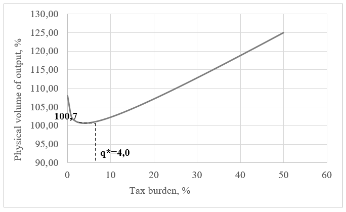
Fig.7 Geometrical interpretation of function (7) for education

This paradox can be interpreted the following way: when a state institution, for example, a university, receives more budgetary and extra–budgetary funds, this inevitably leads to an increase in the cost of its services, which, in its turn, raises the amount of taxes paid. If a university's revenue exceeds a certain minimal level provided by budget funding, this will fuel tax revenue growth and result in a higher tax burden. Thus, it can be concluded that the increasing cost of universities' services results in increasing tax burden. It can be said that there is a reversal of cause and effect: it is not tax burden that influences organizations' activity but, vice versa, their growing activity creates a heavier tax burden. If we take into consideration the fact that state universities are non–profit organizations, we can assume that their whole revenue is distributed to cover the expenses and pay taxes, which causes a faster growth in tax revenue in the growth phase. In any case, changes in the tax burden on universities and schools do not influence their activity, which is mostly determined by the situation on the market.

All the above–said points to the fact that the sphere of education in Russia is unresponsive to tax changes. A rise in the tax burden in this sector neither affects organizations' activity nor makes them increase their turnover to compensate for tax payments. In general, the anomalous form of function (7) signifies that budget-funded organizations of the country's education sector resist standard tax regulation.

Fiscal profile of the health care and social services sector

For a better understanding of the role that the public service sphere plays in the Russian economy, we are going to consider another sector – health care and social services. The procedure is the same as for education. The notation remains the same: F is a dummy variable that takes value F=1 in 2008 and 2016 and in the other years, F=0. The result of our computational experiments based on the data from Table 8 is the following model, which is quite similar to model (6) for electrical engineering:

             (8)

N=14; R²=0.63; DW=2.19; E=0.33%.

Table 8

Input data for model (8) for health care and social services

Model (8) satisfies all the required statistical tests. What distinguishes this model is that the initial fiscal aggregate has a complex form and includes two varying coefficients: W=[lnJ+k*(q–kq²)], where k and k* are varying constants. Dependency (8) is parabolic but is inverted, like function (7). Its maximum point is I*=100.4% with the optimal tax burden q*=5.0% (average lnJ=4.60). For this function, the extreme critical points are economically meaningless (Fig.8). Like education, health care is unlikely to plunge into recession due to increased tax burden. The development of education and health care share the same logic.

Fig.8. Geometrical interpretation of function (8) for health care and social services

Thus, the initial hypothesis that the public service sector will distort the general picture was fully confirmed: in Russia, there are sectors that are either independent of the tax burden or their dependence on the tax burden is anomalous, that is, it cannot be explained from the economic perspective. Therefore, the steady growth of the tax burden in education and health care in the given period does not hold any threat: it is unlikely that they would lapse into a period of stagnation or even recession.

Preliminary conclusions: integral fiscal profile of sectors

The above–described calculations lead us to the conclusions systematized in Table 9.

Table 9

Fiscal profiles of the economic sectors

First, the main indicator that reflects the sectors’ sensitivity to tax regulation is the width of the corridor of acceptable tax burden values (that is, the ones that provide positive production growth): ∆q=q₀₀–q₀. The lower is the value of ∆q, the more sensitive is this or that sector to tax increases. If this is not the case, the degree of the sector's resilience to the increasing tax burden is much higher.

Second, there is a simple but important connection: the more technologically advanced is the sector, the more sensitive it is to tax burden. Table 9 shows that the most vulnerable sector in this respect is electrical engineering, followed by the chemical industry and the manufacturing sector in general, then comes manufacture of coke and petroleum products, with the least vulnerable sector being the extractive industry. It means that tax regulation of new and high–tech industries should be approached with greater care. A possible solution would be to apply lower tax rates to hi–tech industries in comparison with low–tech industries.

Third, there is another interesting pattern: the higher is the technological level of a sector and the more sensitive it is to tax regulation, the more potential it holds in terms of development provided that the fiscal policy is optimal. Table 9 shows that the most impressive growth of production (l*) can be achieved in the electrical engineering sector (7.8% a year) while the potential of the extractive sector is much lower (only 3.1%). To illustrate the potential of these sectors, it is enough to mention that the electrical engineering sector can develop 2.5 times more intensively than the extractive industry. This fact should not be ignored by policy–makers.

Fourth, in the chemical and manufacturing industries as well as in the oil processing industry, the tax burden exceeds the optimal level and any further rise of the tax burden will be detrimental to the development of these sectors. Recently, a similar situation has been also characteristic of the electrical engineering sector. This fact signifies the need for a certain revision or adjustment of the current tax policy.

Our results for the whole economy are worthy of special attention since its sensitivity to tax burden is record–low. It is enough to say that the whole Russian economy is almost 26 times less sensitive to tax tools than the electrical engineering sector alone. While not claiming to provide an exhaustive explanation to this fact, we think that the reasons for this strange fact could be as follows.

First, in our calculations for the whole economy we used GDP as an indicator while for specific sectors, we used the gross amount of revenue. On the macro–level, these indicators differ approximately twofold. Therefore, if we switched from value added to gross revenue, all the fiscal parameters of the Russian economy would decrease approximately twofold: q*=19.3%; q₀=3.8%; q₀₀=34.6%; q=9.5%; ∆q=30.8%. As a result of such calibration of estimates, the economy's sensitivity to tax burden turns out to be almost the same as that of the extractive industry. These rough estimates show that the scale of the paradox described above is not as horrendous as it may initially seem.

Second, technologically, the Russian economy is extremely heterogeneous and comprises multiple industries, which vary substantially in terms of their sensitivity to tax regulation. Judging by the results of our calculations, the aggregation of data for all sectors of economy creates a picture of the economy's generally low sensitivity to taxes. The extractive industry and public service sphere (health care, education, etc) contribute to this situation.

It is quite obvious that an increase in fiscal sensitivity of the Russian economy can be achieved through large–scale restructuring, for instance, by making the country less resource–dependent and, consequently, reducing the share of the extractive industry. Moreover, state clinics and universities should become more economically independent and turn into for-profit institutions partially supported from the public budget.

Discussion: sector-specific differentiated tax burden

The above–described analytical tools enabled us to reveal certain characteristics of development of industries and sectors in relation to their tax burden. Since this is a pilot study, it is aimed primarily at gaining a general understanding of the situation and deals in particular with its qualitative side, that is, the question of whether the tax burden in certain sectors is acceptable or excessive. The idea to apply differentiated tax rates depending on the sectors is highly debatable. Even if we assume that this approach is practically realizable, it would require a variety of conditions to be met. Let us consider some of these conditions in more detail.

The first condition is the reliability of model estimates, which means that the initial input data for a specific industry should be highly accurate. The more detailed this information will be, the better, because this way it will allow us to avoid the one–size–fits–all approach. For example, even the above–discussed electrical engineering sector is quite heterogeneous and includes manufacturing of electrical appliances as well as production of computers involving the use of nanotechnologies. Thus, the first key condition is correct disaggregation of the production output data for specific sectors.

Second, it is necessary to choose the methodology of calculating the average tax burden. In our study, we considered only tax payments of industries although, strictly speaking, we should be summing absolutely all fiscal payments of their enterprises, including numerous payments to extrabudgetary funds (social and medical). We believe that the tax burden on an enterprise should be calculated to include the personal income tax payments since, all other things being equal, increased personal income tax will lead employees to put pressure on their employers calling for a pay rise in order to compensate for their losses caused by the tax increase. In some cases, these losses are borne by employees and in some, they can be shifted to the employer (at least partially). At the same time, it would be desirable that the sum of all fiscal payments in the sector should correspond to gross value added amount, that is, the costs of raw materials, different across the sectors, are not taken into account. If we use value added to calculate the tax burden, then in the right part of the model there should be value added growth indices rather than the cost of goods sold. Thus, all variables in the models should be carefully chosen and their choice should be consistent. In practice, however, this requirement is not met due to the lack of the necessary statistical data.

Third, to make such model calculations practically applicable, it is necessary to ensure that the econometric dependencies themselves should be as accurate as possible. To this end we need, on the one hand, long time series (over 20 years) and, on the other, models should be tested for stability. Moreover, it is advisable to exclude those models that only barely satisfy the main statistical tests. Unfortunately, even these conditions are not met due to the lack of long time series with comparable and detailed statistical data.

Fourth, modelling–based conclusions should be used to draw qualitative conclusions. In other words, it is necessary to estimate whether the effective tax burden exceeds the optimal or critical level or not and if so, then to what extent. Only in the case when calculations show that the situation is serious, the decision should be made to adjust the tax burden. Consensus regarding such adjustments should be achieved through dialogue between representatives of specific sectors and fiscal authorities (FTS).

Fifth, the average tax burden is a parameter that cannot be regulated directly. To increase or reduce the tax burden, adjustments should be made to specific tax rates (VAT, corporate income tax, social security contributions and so on). Therefore, it can be concluded that if model calculations point unambiguously towards the need to reduce the tax burden, this should be achieved in dialogue between industry experts and fiscal authorities. It is also important to take into account the phase in the life cycle of this or that sector which determines the profitability of production and the sector's ability to withstand the tax burden. Tax preferences should be adjusted depending on the phase the sector is in at a certain moment.

Thus, the above–described method is primarily intended for analytical and indicative purposes. Its practical applicability is quite limited and requires that the above conditions should be met.

Conclusion

Our study has shown that the Russian economy is extremely heterogeneous regarding responsiveness of its sectors to different tax regulation tools. The models we built have shown that the current fiscal regime hinders the development in some sectors, which means that for these sectors the tax burden from specifically chosen taxes should be reduced. The most knowledge–intensive and technologically advanced sectors are usually overburdened by taxes, although this fact remains frequently neglected in state regulation practices.

The level of the tax burden in all the sectors we considered is usually within the range of effective values (q₀; q₀₀) and does not exceed the permissible boundaries (except for certain years in some sectors). Therefore, there is no need for a thorough revision of the Russian tax system. What is required is a more delicate adjustment of the tax regime to meet the needs of specific sectors by taking into account the level of technological innovation in these sectors. In its turn, such adjustment implies the principle of differentiated tax rates across sectors. This principle is now applied only to a limited extent even within sectors and we believe that it can be applied more widely. A fitting analogy in this case would be the progressive scale of the personal income tax, which seems quite natural, since we are well aware that different income groups may be more or less sensitive to changing tax rates. There is no reason why a similar principle should not be applied to economic sectors which may be differ significantly in terms of technological intensity and innovation or may be going through different phases of development and, as a result, respond to changes in the tax burden differently. In any case, however, such decisions should be taken only after consensus has been reached between representatives of these economic sectors and fiscal authorities.

References

1. Myles G. Taxation and Economic Growth. Fiscal Studies, 2000, vol. 21, no. 1, pp. 141–168.

2. Andrasic J., Kalas B., Mirovic V., Milenkovic N., Pjanic M. Econometric Modelling of Tax Impact on Economic Growth: Panel Evidence from OECD Countries. Economic Computation and Economic Cybernetics Studies and Research, 2018, vol. 52, iss. 4, pp. 211–226. DOI: 10.24818/18423264/52.4.18.14.

3. Ihendinihu J., Jones E., Emmanuel A. (2014). Assessment of the Long–Run Equilibrium Relationship between Tax Revenue and Economic Growth in Nigeria: 1986 to 2012. The SIJ Transactions on Industrial, Financial & Business Management (IFBM), 2014, vol. 2, no. 2, pp. 39–47.

4. Barro R. Government spending in a simple model of endogenous growth. Journal of Political Economy, 1990, vol. 98, no. 5, part 2, pp. 103–125. DOI: 10.1086/261726.

5. Wanniski J. Taxes, revenues, and the “Laffer curve”. The Public Interest, 1978, no. 50, pp. 3–16.

6. Laffer A., Seymour J. The Economics of the Tax Revoke. N.Y.: Harcourt Brace Jovanovich, 1979. 138 p.

7. Laffer A.B. Government Exactions and Revenue Deficiencies. Cato Journal, 1981, no. 1, рр. 1–21.

8. Laffer A.B. The Laffer Curve – Past, Present, and Future. Heritage Foundation, 2004, article no. 1765, pp. 1–16.

9. Canto V.A., Joines D.H., Laffer A.B. Tax Rates, Factor Employment, and Market Production. The Supply-side Effects of Economic Policy. Economic Policy Conference Series, 1981, vol. 1, pр. 3–32. DOI: 10.1007/978-94-009-8174-4_1.

10. Puljic M. The Application of the Laffer Curve Approach in the Problem of Indebtedness. Available at: http://textfeld.ac.at/pdf/1120.pdf

11. Papava V. Laffer’s Effect with After–Action. World Economy and International Relations, 2001, no. 7, pp. 34–39. (In Russ.).

12. Stuart C. Swedish Tax Rates, Labor Supply and Tax Revenues. Journal of Political Economy, 1981, vol. 89, pp. 1020–1038. DOI: 10.1086/261018.

13. Feige E.L., McGee R.T. Sweden's Laffer Curve: Taxation and the Unobserved Economy. The Scandinavian Journal of Economics, 1983, vol. 85, no. 4, рр. 499–519. DOI: 10.2307/3439948.

14. Ravestein A., Vijlbrief H. Welfare Cost of Higher Tax Rates: An Empirical Laffer Curve for the Netherlands. De Economist, 1988, no. 136, рр. 205–219. DOI: 10.1007/BF01238621.

15. Heijman W.J.M., Ophem J.A.C. Willingness to pay tax: The Laffer curve revisited for 12 OECD countries. The Journal of Socio–Economics, 2005, vol. 34, iss. 5, pp. 714–723. DOI: 10.1016/j.socec.2005.07.013.

16. Strulik H., Trimborn T. Laffer Strikes Again: Dynamic Scoring of Capital Taxes. European Economic Review, 2012, vol. 56, iss. 6, pp. 1180–1199. DOI: 10.1016/j.euroecorev.2012.05.002.

17. Trabandt M., Uhlig H. The Laffer Curve Revisited. Journal of Monetary Economics, 2011, vol. 58, iss. 4, pp. 305–327. DOI: 10.1016/j.jmoneco.2011.07.003.

18. Lin B., Jia Z. Tax rate, government revenue and economic performance: A perspective of Laffer curve. China Economic Review, 2019, vol. 56, article 101307, pp. 1–20. DOI: 10.1016/j.chieco.2019.101307.

19. Hearne A.I., Svidnytskyy T.I. Modeling Effect in Economics Laffer Ukraine Industrial and Institutional Functions. Financial and credit activity: problems of theory and practice, 2013, no. 1(14), pp. 115–123. (In Ukr.).

20. Gusakov S.V., Zhak S.V. Optimal Equilibrium Prices and the Laffer Point. Economics and Mathematical Methods, 1995, vol. 31, iss. 4, pp. 346–358. (In Russ.).

21. Canto V.A., Joines D.H., Webb R.I. The Revenue Effects of the Kennedy and Reagan Tax Cuts: Some Time Series Estimates. Journal of Business & Economic Statistics, 198, vol. 4, no. 3, pp. 281–288. DOI: 10.2307/1391570.

22. Stiglitz J. The Roaring Nineties: Seeds of Destruction. London, 2003. 389 p.

23. Malcomson J.M. Some analytics of the laffer curve. Journal of Public Economics, 1986, vol. 29, no. 3, pp. 263–279. DOI: 10.1016/0047-2727(86)90029-0.

24. Fullerton D. On the possibility of an inverse relationship between tax rates and government revenues. Journal of Public Economics, 1982, vol. 19, iss. 1, pp. 3–22. DOI: 10.1016/0047-2727(82)90049-4.

25. Mirowski P. What’s Wrong with the Laffer Curve? Journal of Economic Issues, 1982, vol. 16, no. 3, pp. 815–828. DOI: 10.1080/00213624.1982.11504034.

26. Balatskii E.V. The Influence of Fiscal Instruments on Economic Growth: An Evaluation. Studies on Russian Economic Development, 2004, vol. 15, no. 4, pp. 412–419. (In Russ.).

27. Mayburov I. A., Sokolovskaya A. M. The theory of taxation. Advanced course. Moscow: Yunity–Dana; 2011. (In Russ.).

28. Papava V. The Georgian Economy: from «Shock Therapy» to «Social Promotion». Communist Economies & Economic Transformation, 1996, vol. 8, no. 2, pp. 251–267. DOI: 10.2139/ssrn.2182406.

29. Ananiashvili Iu., Papava V. Laffer-Keynesian Synthesis and Macroeconomic Equilibrium. Stockholm: CA&CC Press, 2010. 142 p. (In Russ.).

30. Ananiashvili Iu., Papava V. Taxes, production technology and economic growth. Society and Economy, 2011, no. 4–5, pp. 172–196. (In Russ.).

31. Ananiashvili Iu., Papava V. Impact of the Average Tax Rate on the Aggregate Demand (Keynesian Models). Bulletin of the Georgian National Academy of Sciences, 2012, vol. 6, no. 2, pp. 162–169.

32. Sokolovskaya A.M. Methodological and methodical aspects of determination of the tax burden on labor, capital and consumption. Finance of Ukraine, 2008, iss. 1, pp. 65–76. (In Ukr.).

33. Bukach B.A. Substantiation and analysis of various variants of the graphic interpretation of the Laffer curve. Vestnik SevNTU, 2012, no. 130, pp. 30–38. (In Russ.).

34. Gutmann P. The Subterranean Economy. Financial Analysis Journal, 1977, vol. 33, no. 6, pp. 26–34.

35. Henderson D. Limitation of the Laffer curve as a justification for tax. Cato Journal, 1981, vol. 1, no. 1, pp. 45–52.

36. Becsi Z. The Shifty Laffer Curve. Federal Reserve Bank of Atlanta. Economic review, 2000, vol. 85, no. 3, pp. 53–64.

37. Balatskii E.V. Using Production–Institutional Functions to Analyze the Influence of Tax Load on Economic Growth. Studies on Russian Economic Development, 2003, vol. 14, no. 2, pp. 134–144. (In Russ.).

38. Kakaulina M. Graphic Interpretation of the Laffer Curve with Tax "Migration". Bulletin of Ural Federal University. Series Economics and Management, 2017, vol. 16, no. 3, pp. 336–356. DOI: 10.15826/vestnik.2017.16.3017.

39. Movshovich S.M., Sokolovsky L.E. Issue, taxes and the Laffer curve. Economics and Mathematical Methods, 1994, vol. 30, no. 3, pp. 129–141. (In Russ.).

40. Bukach B.A. Analysis of the main assumptions of the Laffer curve. Vestnik SevNTU, 2011, no. 116, pp. 17–24. (In Russ.).

41. Kakaulina M. Tax burden and economic growth: search for an effective model. Tomsk State University Journal, 2015, no. 394, pp. 181–188. DOI 10.17223/15617793/394/30. (In Russ.).

42. Kakaulina M. Influence of Tax Burden on Economic Growth in the Russian Federation: a Regional Aspect. Regional Economics: Theory and Practice, 2014, no. 17(344), pp. 55–64. (In Russ.).

43. Nikulina O.M. Tax burden in Russia: basic approaches. Finance and Credit, 2016, no. 17 (689), pp. 13–27. (In Russ.).

44. Turbina N.M., Kosenkova Yu.Yu. Tax burden as indicator of effectiveness of tax policy of Russia. Social and Economic Phenomena and Processes, 2017, vol. 12, no. 2, pp. 154–159. DOI: 10.20310/1819-8813-2017-12-2-154-159. (In Russ.).

45. Kakaulina M. Assessment and Analysis of the Fiscal Burden in the Russian Federation: An Industry Aspect. Tomsk State University Journal, 2019, no. 46, pp. 189–205. DOI:10,17223/19988648/46/13. (In Russ.).

46. Balatsky E., Ekimova N. Tax-Budget Policy and Economic Growth. Society and Economy, 2011, no. 4–5, pp. 197–214. (In Russ.).

Official link to the article:

Balatsky E.V., Ekimova N.A. Evaluation of Russian Economic Sectors’ Sensitivity to Tax Burden // «Journal of Tax Reform», Vol. 6, no. 2, 2020, pp. 157–179.