Introduction

Over the last several years, the status of the Central Bank of the Russian Federation (CBRF) has changed from macroregulator to megaregulator. Thus, the conventional concept of a regulator (macroregulator) implies executive authority, which directs the development of the national economy in terms of its specific segments. As a rule, a macroregulator has a broad, yet limited area of activity and a regulated object, while a megaregulator possesses advanced authorization in managing the regulated object, the latter is extremely broad. Today, only the CBRF is a fully capable megaregulator in Russia.

In modern economic policies and practices, questions and answers regarding the evaluation of the influence of the country’s monetary area on economic growth are relevant [1, 2], along with determining the efficiency of operations of the Bank of Russia [3, 4].

A particular monetary policy (MP) was discussed in the studies of the so–called monetary rules (MRs), where the central bank assumes certain obligations and acts in accordance with the established algorithms of the monetary policy. However, the MRs are currently deemed too narrow in terms of the regulatory needs of the monetary authorities, for which reason the so–called macroprudential policy becomes established, which means using the prudential tools in order to reduce the risk in the financial sector, particularly the constraints of bubbles on the financial and loan markets [5].

Various additional tools are being developed as part of this widening approach to the MPs that produce the effect of early crisis prevention. For example, the Center for Macroeconomic Analysis and Short–Term Projection (CMASP) of the Institute of Economic Forecasting of the Russian Academy of Sciences forms summary anticipatory indices (SPIs) across various lines of study on a monthly basis [6]. As of 2012, the CBRF has been publishing the Financial Stability Review twice a year, which contains the analysis and evaluation of the key financial markets, which not only belong to the Russian financial system and its individual sectors, but also to the global economy and financial markets [7]. From the fourth quarter of 2007 until the second quarter of 2011, the Gaidar Institute of the Economic Policy published The Financial Stability Monitor every month based on the corresponding indicators [8, 9]. The Analytical Credit Rating Agency (ACRA) has developed and publishes the Financial Stress Index for the Russian Federation daily [10]. In 2012, the Center for Macroeconomic Studies of Sberbank of Russia developed a weekly Index of Financial Stability (IFS) for Russia, which was intended as a means to regularly track the state of the country’s financial system [11].

In order to estimate the influence of financial indicators on the economic growth, the authors of [12] studied the effects of such indicators as the internal loan market (ratio of the bank loans to the private sector to the GDP), the internal market of corporate bounds (ratio of the volume of the internal corporate bounds to the GDP), and the market of external corporate debt (ratio of the external corporate debt to the GDP) on the economic growth rate and macroeconomic stability. In [13], the MP efficiency of the Bank of Russia is analyzed based on modeling the mid–term economic dynamics amidst different scenarios of the changing key interests.

However, the wide practice of applying various anticipatory indicators revealed the generally acknowledged leader, the use of which can be circulated at its maximum, yet did not allow the most effective methods and models to be determined. As such, the need to build some sort of aggregated, summary indicator of the monetary climate arises that could be used, first, to diagnose the current MP and its efficiency and, second, to predict the economic growth several months in advance. The creation of this particular indicator is the goal of this study.

Ideology of building the index of monetary efficiency

Currently, the Bank of Russia has accumulated a large array of quite useful information about the money–and–credit processes in the country. In this context, many indicators of the monetary statistics are provided every month, which creates a basis for effective monitoring the monetary climate. However, all of these indicators are disparate and do not enable a holistic evaluation of the real situation. The major idea of this work is to build such a summary index that would accumulate all the main parts of the money–and–credit processes and allow changes in the monetary climate to be tracked on a timely basis.

The suggested index of monetary efficiency (IME) must have two properties, i.e., both structural and dynamic effectiveness. The structural effectiveness resides in the presence of two components in IME, one of which characterizes the monetary stability, while the other characterizes monetary freedom. The dynamic effectiveness resides in the quality of IME as an anticipatory indicator that provides advanced notice of any further negative processes in the real economy.

The above–mentioned structural property is based on D.North’s thesis regarding the duality of the institutions, which create both limitations and stimuli [14]. This means that the institutions must possess two discordant properties, i.e., rigidity and flexibility. According to the definition by D.North, in which institutions set the rules of the game, and the definition by V.M.Polterovich, in which institutions set the norms of behavior [15], one can conclude that the Bank of Russia is a typical regulator institution, which sets standard rules of the game and the norms of behavior for the participants of the money–and–credit system. As such, the activity of the Russian megaregulator possesses the duality described by D.North. According to the political theory of D.Zolo, a state that performs the regulation process must that diametrically opposed values of the safety and freedom of its civilians are balanced [16]. In this case, the Bank of Russia must ensure the reliability (security) of the money and credit systems, as well as the stimuli (freedom) of the activity of economic agents.

The aforementioned methodological tools underwent instrumental refinement during the process of building the Basic Index of Institution Development (BIID), which was formulated in 2015 at the Financial Institute under the Government of the Russian Federation [17, 18]. In particular, when devising the BIID, the safeguards and freedoms provided by the national institutions were examined, as a result, the target index was broken down into the index of institutional safeguards and the index of institutional freedoms. The given approach was finalized by digitizing all aspects of the two institutional lines of development, which allows the created analytical technique to be classified as an extremely promising and replicate it in other areas of institutional studies. As such, considering the Bank of Russia to be a regulating institution and the monetary climate to be the result of this regulation, it is reasonable to use the stated functional gradation of institutions in the context of safeguards and freedom. In this case, the general monetary efficiency is formed based on monetary stability and monetary freedom. Correspondingly, the Index of Monetary Efficiency (IME) will comprise two specific indices, i.e., the Index of Monetary Stability (IMS) and the Index of Monetary Freedom (IMF). The suggested approach is relevant from the viewpoint of the MP regulation because the activity of the megaregulator often notably shifts toward introducing limitations and pursuing the stabilization of the situation, while the tools of stimulation are almost completely offline. A reasonable balance between the two sides of regulation is achieved more easily if there is a responsive indicator like the IME and its components.

Calculating the index of monetary stability

In order to balance the effects of the limitations (stabilization) and releases (freedoms), the specific indices, IMS and IMF, shall consist of equal amounts of the initial reporting indicators. In our case, each particular aggregate has seven assumed elements. For the purpose of clarity, the architecture of the IMS is shown in Table 1.

Table 1. Elements of the Index of Monetary Stability (IMS), %

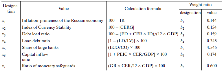
In Table 1, please refer to the following designations: IR is the monthly inflation rate (inflation is subtracted from 100 to normalize the general calculation logic, which implies that a higher value of the parameter is better); CERG is the monthly growth of the currency exchange rate, USD (the indicator is in absolute magnitude to account for the absolute scale of change regardless of the direction); ID/ED are the internal and external state debt, RUB; CER is the currency exchange rate USD/RUB; GDP is the monthly value of GDP (multiplied by 12 to convert the monthly value to annual), RUB; LD is the loan debt of resident legal entities and private entrepreneurs, RUB; LV is the loan volume, RUB; CO is the number of large credit organizations in the country; LCO is the number of large credit organizations with a registered capital of 10 billion RUB; PIEC is pure import (+) and export (–) of capital (subtracting from 1 enables the sign of net data to be eliminated and the general logic of the results to be valuated; the higher the indicator the better), USD; GR is global reserves, USD. All indicators are based on the monthly statistics of the Bank of Russia except for monthly values of the GDP, which were provided by Vnesheconombank (VEB). The retrospective series used in the applied calculations includes data for October 2014 to March 2017, i.e., 30 monitoring points.

The indicators below are used to evaluate the reliability of the monetary system; low values indicate an increase in the probability of any form of a crisis. Considering that all seven indicators cannot change synchronously, they should be aggregated by a certain rule. There is no explicit algorithm for this aggregation, due to which a quite operational method, which is also the simplest, can be proposed that consists of the following. It is necessary to select the weight ratios such that, at the initial time moment, the IMS value equals 100%. Then, looking at its further dynamics, one can presume an improvement (or deterioration) of the situation as compared to that in the initial moment of time. Having this said, IMS does not have any valuation and does not reside within any strictly defined limits. On the contrary, its value varies around 100%, and its lower and upper boundaries are not fixed. Thus, one can only discuss the historical minimums and maximums of IMS.

The general formula of IMS looks as follows:

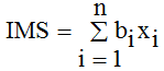         (1)

where b_i is the weight ratio of the ith specific indicator of monetary stability and n is the number of indicators (in our case, n = 7).

The basis of the algorithm for finding the weight ratios is the rule, which implies that all specific indicators contribute equally to the overall aggregate of IMS. Then, the weight ratios are found from the following equation:

                    (2)

The calculations result in a number of weight ratios, i.e., b₁ = 0.144; b₂ = 0.154; b₃ = 0.159; b₄ =0.345; b₅ = 4.545; b₆ = 0.174; b₇ = 0.600 (see Table 1).

We must highlight that the used approach to calculating the weight ratios is aimed at aligning the scale of the effect produced by each factor and does not reveal its role based on the weight. On the contrary, a difference in the weight ratios automatically reflects the difference in the scale of factor indicators. This is why the weight ratios are not subject to conventional valuation.

It is worth mentioning that the number of explaining factors of IMS do not contain the parameter of the reservation norm, which is traditionally viewed as an important tool of central banks. This is justified because the circumstances under which this tool changes its value are particularly rare; the Bank of Russia can remain constant for several years. Apparently, the given parameter has achieved some optimal value in today’s age, and its active involvement in the nearest future is unlikely. As such, the reservation coefficient has actually become a secondary backup tool for macroprudential policy and, hence, its exclusion from the composition of IMS at the current phase can be substantially justified.

Calculating the index of monetary freedom

In order to calculate IMF, the entire procedure of calculations is similar to that used for IMS. The aggregate of IMF also includes seven parameters. For the sake of clarity, the architecture of IMF is shown in Table 2. As with the IMS index, the retrospective series includes statistics for October 2014 through March 2017.

Table 2. Elements of the Index of Monetary Freedom (IMF), %

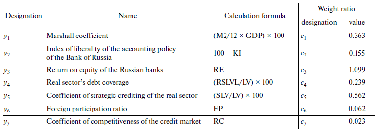
In Table 2, please refer to the following designations: М2 is the standard money aggregate М2, RUB; KI is the key interest of the Bank of Russia, %; RE is the average return on equity of the credit organizations in Russia, %; RSLV is the number of loans to the real sector of the economy, RUB; SLV is the strategic loans volume, i.e., the amount of loans to the real sector over a term of more than 3 years, RUB; FP is the number of credit organizations with foreign participation in the registered capital; RC is the number of Russian credit organizations.

All of the listed indicators evaluate the freedom of actions taken by the economic subjects of the country when working with the loan system; if they show poor (low) values, it can act as a restraint for developing the national economy.

The general formula of IMF looks as follows:

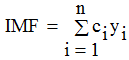                                                                                           (3)

where c_i is the weight ratio of the ith specific indicator of monetary freedom and n is the number of indicators (in our case, n = 7).

The calculations by scheme (2) result in a number of weight ratios: с₁ = 0.363, с₂ = 0.155, с₃ = 1.099, с₄ =0.239, с₅ = 0.562, с₆ = 0.062, and с₇ = 0.023 (Table 2).

After determining IMS and IMF, the problem of calculating IME becomes trivial and can be solved by the simple averaging of the following two indices:

                                                                (4)

According to (4), the stability and freedom are of equal significance to the monetary efficiency. This seems quite justified from both general theory (no phenomenon must be given preference) and instrumental (equal numbers of factors in each subindex) points of view.

Special mention should be made of the aspect related to a possible nonlinearity of the effects discussed in the previous section. For example, under regular conditions, the growth in the ratio of the real sector’s debt coverage (y₄) plays a positive role that reflects the sufficient monetary policy of the national economy. However, as was mentioned before, excessively high values of this ratio may create conditions for the destructive inflation of the bubble, which indicates the artificial nature of production stimulation. In the future, this circumstance may affect the estimation of the influence of IME on the GDP; however, we are ignoring this aspect of the problem because, in Russia none of these parameters has ever approached the line where the negative effects of intense credit activity start to manifest.

Empirical results of the calculation of the index of monetary efficiency

The results of the calculation of indices IMS, IMF, and IME are shown in Fig.1. In particular, the trend of persistent growth of IMS is vivid. Thus, during the entire studied period, the deterioration of this index as compared to the initial value equal to 100% (of November 2014) was only observed in April 2015, while in the other months, the IMS dynamics showed a prevalence of growth.

As a result, by the end of the retrospective period (February–March 2017) its value had grown by approximately 16–17% relative to the initial value (Fig.1a). This indicates the implementation of the focused policy of the Bank of Russia for improving the stability of the money and-credit sphere, which also indicates IMS. This trend continues to persist.

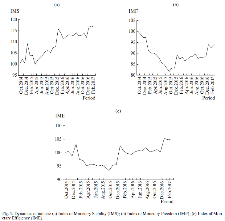
As for IMF, a diametrically opposed trend is observed (Fig.1b). The events in Crimea and subsequent currency crisis gave rise to the process of restricting monetary freedom. This trend bottomed out around one year later, in November 2015, when the IMF value decreased by more than 18% (Fig.1b). Then, the situation began to improve slowly but surely. However, even by February 2017, the IMF was still 6% lower than in November 2014. Thus, the processes of the 2014–2016 crisis contributed to an asymmetric monetary policy, which was aimed at tightening control over and achieving stabilization by reducing economic freedoms. In our opinion, under the current circumstances, there was no reasonable alternative to this policy.

The IME dynamics was decreasing during the entire year of 2015, which is quite understandable given that international sanctions and the collapse of the ruble required the enhancement of monetary regulation and reduced all kinds of financial freedom. The maximum drop in the IME was 6.5%, which can be classified as a rather moderate decline in the monetary climate considering the particular economic conditions (Fig. 1c). However, in 2016, the IME started to grow sustainably. The maximum growth by March 2017 was a little more than 5%. In general, the trend of the monetary efficiency to grow prevailed and, hence, the regulation crisis came to an end and, at present, some small but tangible progress has been achieved.

One important comment should be made regarding the sensitivity of the indices that have been built. The matter is that the volatility of the IMS and IMF indices is not too high; the IME possesses even more inertia due to the differently directed trends between the aggregates that comprise it. For example, the initial value of the indices 100% cannot increase by two or three times; according to the observations, all changes are within ±20%. This is conditioned by the structure of the indices itself and the weight ratios, which exclude excessively intense fluctuations. This means the high cost of each percentage–based item of the changes. This way, if the index grows (or declines) by 10%, it is actually a massive number that indicates serious changes to the monetary climate. Below, we will return to this topic and discuss it in more detail.

Comparing the dynamics and absolute values of IMS, IMF, and IME with the previously constructed indicators of the institutional effectiveness, institutional safeguards [17], and institutional freedom is extremely informative. It turns out that not only Russia, but also all post-Soviet countries were prone to covering quite large institutional safeguards amidst the lowered institutional freedoms.

In this case, we obtained the same result. The Bank of Russia primarily ensures the monetary stability, while providing monetary freedoms becomes secondary for it. On one hand, this fact indicates the existence of a quite objective regulation pattern, which resides in the immediate stabilization of the situation with the further loosening of the restrictions, which leads to growth in the market freedoms of economic agents. On the other hand, in this case, a sort of management cliche is observed, which is targeted at restraining market freedom for an extremely long period of time. Apparently, this format of regulation is based on the fact that Russia belongs to a type of countries, in which safeguards have played the role of a primary good and freedom has been viewed as an additional secondary good for a long time.

Index of monetary efficiency and ideology of the anticipatory indicator

The constructed IME and its components has analytical self–value because its use allows not only the comfort of the monetary climate and the effectiveness of the CBRF’s actions to be assessed, but also the driving forces of the occurring changes to be decrypted in a unique way. Monitoring the dynamics of the IME allows not only the improvement or decline of the monetary situation to be diagnosed, but also the imbalances of management in the activity of CBRF. In this sense, IME may be used in the autonomous analytical mode without additional operations. However, the index also possesses an additional value, which lies in the fact that it can be used as an anticipatory indicator of future economic growth. In this case, it is assumed that IME first must be linked to the monthly value of GDP by its economic dependence and, secondly, this dependence of the GDP on IME must have some lag; the second indicator shall fall at least several months behind the first one. In this case only, the prompt diagnostics of the monetary climate through INE will enable short–term projections regarding the expected changes in the GDP.

The set goal of constructing an econometric model of the lag between the GDP and IME is broken down into two phases. The first phase consists of constructing the simplest possible aggregated dependence between the GDP and IME, with the letter aimed at disclosure, as well as detailing the dependence such that the GDP depends on both monetary aggregates, i.e., the IMS and IMF. The first model is basic. It is used to determine whether there is dependence and understand its basic properties. The second model allows for a more in–depth calibration of the obtained dependence and, thus, to improve the accuracy of the applied calculations and draw additional analytical conclusions. Moreover, the GDP should be predicted using the second model due to its more appropriate approximation.

The models enable predictions at both the qualitative and quantitative levels. For example, if there is a lag of several months between the GDP and IME, one can use any explicit declines (increases) in the IME dynamics as a basis, on which the similar declines (increases) in the GDP can be predicted, thus projecting some events at the qualitative level. If a more refined model is used, which represents a recurrent relation, it can be used to obtain future (several months ahead) values of the GDP and specific values for the further production activity of the system, i.e., a short–term quantitative prediction.

Basic econometric model of growth

A particular feature of the econometric model is that is has a time lag, the value of which is not known in advance. As such, constructing the model implies performing numerous computational experiments, in process of which that the lag is shifted from 1 to 12 months.

The dependence to be found is built as a linear regression between the GDP (or its logarithm) and IME with a lag of h months based on monthly data t as follows:

             (5)

where α and β are the econometrically estimated model parameters.

Dependence (5) suggests a simple institutional function of the economic growth as an exponent from the monetary climate as follows:

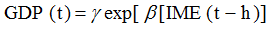
where γ=e^α is a constant.

The applied calculations allowed the following dependence to be determined:

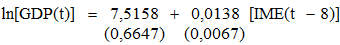 (6)

N=22; R²=0,173; DW=1,464; E=7,07%

The corresponding standard errors are given in brackets under the regression ratios; N is the number of observations, R² is the coefficient of determination, DW is the Durbin–Watson statistic, and E is the approximation error.

The built model undergoes the main statistical tests and provides a satisfactory level of approximation. Thereby, model (6) gives an explicit answer regarding a relation between the dynamics of GDP and the constructed IME. In this context, the time lag is 8 months, which provides for a good basis for proactive projection.

The obtained result converges with the fundamental a priori statements. In fact, the monetary climate must influence the economic growth, which is shown by model (6). At the same time, it is obvious that the influence of the monetary climate cannot be defining, which is also reflected in the model, the proportion of explained dispersion is 17%, while the remaining 83% of changes in the GDP are produced by other factors not considered in the model.

Model (6) allows for the most generalized understanding of the monetary factor. For example, a simple dynamic relation can be derived from (6) as

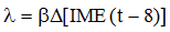(7)

where λ is the rate of economic growth.

Knowing that β = 0.014, one can conclude that the growth of the index of monetary efficiency by 10 points can increase the rate of economic growth by 1.4% If the IME value has not reached its limit, then its increase suggests notable reserves for the growth in the national economy. And although the monetary factor by itself cannot ensure the Chinese rates of economic growth for Russia (∼10% annual), it can still energize the economy and provide sustainable nonzero growth. This is one of the main conceptual results of the model.

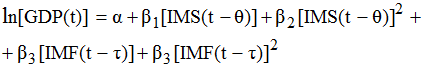
It is worth mentioning that, even in simplified form, model (6) takes into account both aggregates of the IME (IMS and IMF). This is directly implied when this model is expanded as follows:

                   (8)

However, the given dependence requires detailing, which serves several purposes. First, it is reasonable to assume that IMS and IMF affect the economic growth differently in terms of intensity, and this difference should be determined as a quantitative measure. Second, there are reasons to believe that IMS and IMF influence the dynamics of GDP with a lag of different durations, which requires verification. Third, it is quite possible that the influence of IMS and IMF is of a nonlinear nature with all the resulting consequences, which also requires verification. Fourth, it is reasonable to have a model that explains a much larger percentage of the GDP changes than dependence (6).

As such, it is legitimate to set the problem of constructing some modification of model (6), which would satisfy each of the four requirements above.

Additional (supplementary) econometric model of growth

In order to solve the set problem and obtain a more saturated analytical structure, we built the following nonlinear factor-based model:

                                (9)

where θ is the time lag between the GDP and IMS and τ is the time lag between the GDP and IMF.

The approbation of the model allowed it to be determined that θ = 3 months and τ = 11 months, and the following econometric model to be obtained:

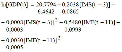                                       (10)

N=19; R²=0,702; E=3,90%.

The model undergoes the main statistical tests and provides a high level of approximation. The resulting dependence possesses a number of properties and contains quite a lot of additional information.

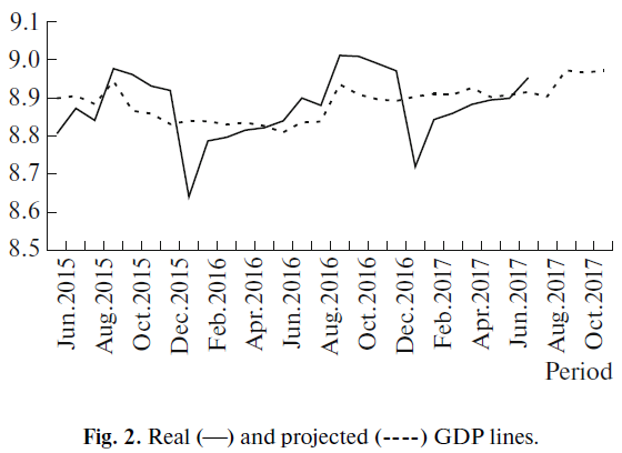
First, model (10) provides higher accuracy in terms of both insignificant approximation error and a higher coefficient of determination; other factors define less than 30% of all changes in the GDP. These qualities allow model (10) to be used to directly predict the GDP dynamics. Second, the hypothesis regarding the influence of IMS and IMF on the GDP dynamics with different lag durations proved to be true. The coefficient of stability affects the GDP dynamics within as little as 3 months, while the shifts in the coefficient of freedom affect it 11 months later. This conclusion is independent of understanding the process of state regulation and its priorities. The matter is that all measures of monetary stabilization affect economic growth very quickly, while the provision of monetary freedoms affects the GDP positively, but the result is observed a little less than a year later. As such, it is not surprising that in most cases, the regulator gives preference to restricting measure of stabilization instead of liberal ones based on the maximum release of the loan market. An extended response of the system to the monetary freedoms holds certain dangers related to the fact that unexpected events can occur during this period, which will nullify the liberal effect. Thus, the observed anticipatory dynamics of IMS (Fig.2a) compared with the decline dynamics of the IMF (Fig.2b) represents a natural reaction to the deteriorating economic conditions. An important result of the analysis is an intuitive approach to the effect of safeguards and freedoms on the economic growth, which was explicitly confirmed, empirically transforming it from a hypothesis to a confirmed fact. Third, the influence of IMS and IMF on the GDP is actually of a nonlinear nature, which provides new analytical possibilities.

The first thesis derived from model (10) is based on the presence of a parabolic dependence between the GDP and IMS with a maximum point for IMS* as follows:

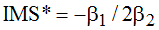 (11)

This means that the policy that growth in monetary stability has a natural upper limit and exceeding it deteriorates, rather than improves the situation. The calculations show that this point is IMS* = 122.5%. Therefore, it is reasonable for the Bank of Russia to plan its regulatory actions such that the set boundary is not exceeded. The main conclusion is that the superfluous activity of the regulator on restraining the activity within an industry is of a destructive nature; there is a possibility of strangling the economy in a vice of excessive monetary requirement. The analysis of empirical data of the IMS indicates that the given regulation reserve is not yet depleted, since the actual values of IMS have never exceeded the critical value of IMS*. Currently, the Bank of Russia has a significant reserve (5 percentage points) in enhancing the stabilizing actions.

The second thesis concerns the presence of a parabolic dependence between the GDP and IMF with a minimum point for IMF* as follows:

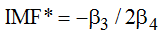 (12)

This means that the policy of growth of the monetary freedom has a natural lower limit, and when it is reached, the situation deteriorates. The calculations show that this point is IMF* = 88.8%. Therefore, the Bank of Russia must execute a policy in which monetary freedoms are not below the stated level, as in the case with point (12), the window of opportunity can be closed for economic subjects. The analysis of the factual data shows that this requirement has been systematically violated. Thus, in June 2015 to December 2015, February 2016 to July 2016, and September 2016 to December 2016, the value of IMF was below the calculated critical boundary. The values of the IMF only left the dead zone in 2017, and the liberalization and release of the loan system were initiated.

The third thesis is that the main regulatory reserve of the Bank of Russia is in the area of accumulating the monetary freedoms and very slight pressure towards the market stabilization. In the long run, the growth of IMF must become the driver of improvement for the monetary situation in the country.

The fourth thesis implies returning to the discussion about the boundaries of change in the IMS and IMF. As was stated before, the deviation of their actual values from 100% is within ±20%. The completed analysis allows refining this conclusion. In particular, the upper limit for IMS is 122.5%, and, roughly speaking, the lower one is not defined. For IMF, the lower limit is 88.8%, i.e., 1102 percentage points lower than initial point 100%, while the upper limit is also not defined. It is most likely that the movement of IMS toward the bottom is about the same value as toward the top, i.e., about 22%; likewise, the movement of IMF toward to top cannot exceed 15 percentage points. Thus, the range of the constructed indices is quite limited. The overrun will indicate the necessity of a thorough analysis of efficiency of monetary regulation.

Retrospective and perspective projection

The constructed basic model (6) allows predicting the value of the monthly GDP for 8 months ahead. In this context, in order to evaluate the accuracy of prediction, the socalled retrospective projection can be performed based on the reporting data. In this case, the result is known in advance and is characterized by approximation error for dependence (6). However, perspective projection is also possible, in which formula (6) is used to recalculate the GDP for 8 months ahead. This procedure was performed and produced quite a satisfactory result (Fig.2). In this case, the main question is the degree of credibility of these projections. In order to answer this question, we ran a conventional test, i.e., a comparison of the obtained prediction data with the reporting data obtained later.

Considering the fact that the starting point was March 2017, the projection covered the period until November 2017. After some time, we obtained new data on the GDP from Vnesheconombank for four reporting months. This allowed the previous projection results to be compared with the actual data on the GDP obtained after them (Table 3).

Table 3. Comparing planned and real values of the GDP

The results are promising because the average error of the predicted values for four months is 2.4%, which is significantly lower than the fixed error of approximation for model (6). Thus, the long-term results of model (6) are more than satisfying. As such, the use of more refined dependence (10) is pointless.

It should be noted that the accuracy of the prediction can be additionally improved by taking into account the recurrence of the monthly GDP. The model values smoothen the recurrent spikes, which must be generated by a special operator.

Aside from simple projections of monthly GDP volumes, model (6) allows the assumed annual growth of GDP to be evaluated if necessary. To do this, the following value should be determined as follows:

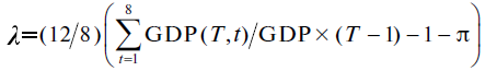(13)

where λ is the rate of economic growth, GDP(T, t) is the produced GDP in the tth month in current year T, GDP(T – 1) is the produced GDP in previous year T– 1, and π is the anticipated annual index of inflation in the current year.

The calculations by formula (13) based on Table 3 provide the value of the rated GDP as 5%, and, considering the annual inflation expected by the Bank of Russia as 4%, determine the value of the anticipated rate of the real growth of GDP in 2017 to be 1%.

Thus, the constructed IME with the accompanying model (6) can become an operational tool for short–term projection of the production activity in Russia.

CONCLUSIONS

The use of the index of monetary activity in the practice of state regulation. The developed analytical tools, i.e., the IME, IMS, and IMF monetary indices, as well as basic and supplementary econometric models for proactive diagnostics, are designed for strategic and tactical applications.

Strategic applications are aimed at determining and adjusting the global course of monetary regulations by the CBRF. For example, in recent years, the predominant activities of the Bank of Russia were to stabilize and restrain, while stimulation policy was secondary. In our opinion, in the next 1–1.5 years, this situation may continue and yield positive results. However, in the long run, but no more than 2 years, the strategy of the CBRF must change dramatically, and the regulator will have to utilize tools for stimulating the monetary area more actively, which will most likely provide a new source of economic growth in Russia. Otherwise, excessively tight and repetitive restraining actions of the Bank of Russia will hinder the development of global monetary events and crises without allowing the potential activity of domestic economic subjects to come to fruition. It is obvious that certain terms and measures of revising the priorities in the CBRF’s policy are the prerogative of the megaregulator’s management and are defined according to the macroeconomic context.

The tactical application of the developed tools implies using two principally different approaches, i.e., internal and external. Both approaches suggest the systematic monitoring of the IME, IMS, and INF indices, as well as constantly updating basic and supplementary econometric models of proactive prediction, specifications, and parameters. This monitoring of the monetary situation and its efficiency will allow for monthly projections of the GDP up to 8 months in advance. In a number of cases, these projections will enable the timely identification of any emerging crisis, and the anticipatory period of 8 months can be used to elaborate stabilization measures. The difference between the first and second approach is that the internal mode is oriented toward performing accounting, analytical, and prediction operations within the regulator itself in the CBRF, while the external mode implies that this work was performed by a third party with a higher status and analytical capability. Each of these approaches has its benefits and drawbacks, and preferring one of them is a matter of context, not a scientific problem.

ACKNOWLEDGMENTS

This article was prepared as part of the State Assignment from the Government of the Russian Federation to the Financial University under the Government of the Russian Federation for 2017 (project no. AAAA-A17-117060110148-8 “Development and Analytical Support of the Index of Monetary Efficiency in the Russian Federation”).

REFERENCES

1. V.S.Panfilov, O.Dzh.Govtvan’, and A.K.Moiseev, “Finance and credit in the strategy for the economic development and structured investment policy of the Russian Federation,” Stud. Russ. Econ. Dev. 28 (6), 575–584 (2017).

2. V.S.Panfilov, Financial and Economic Forecasting: Methodology and Practice (MAKS Press, Moscow, 2009) [in Russian].

3. O.Dzh.Govtvan’, Methodology and Experience of Forecasting the Russian Monetary and Banking System (MAKS Press, Moscow, 2009) [in Russian].

4. V.S.Panfilov and O.Dzh.Govtvan, “Russia’s financial policy in the perspective period,” Stud. Russ. Econ. Dev. 23 (6), 556–567 (2012).

5. The role of macroprudential policy in the context of correlating commodity cycles with capital flows and the financial cycle: An analytical note of the Financial Stability Department of the Bank of Russia, The Central Bank of the Russian Federation, August 2017. http://www.cbr.ru/Content/Document/File/16743/analytic_note_170808.pdf.

6. Consolidated Leading Indicators of Systemic Financial and Macroeconomic Risks, Center for Macroeconomic Analysis and Short–Term Forecasting (2017). http://www.forecast.ru/default.aspx.

7. Review of financial stability, Central Bank of the Russian Federation (2017). http://www.cbr.ru/publ/?PrtId=stability&pid=fin_stab&sid=ITM_31265.

8. P.V.Trunin and M.V.Kamenskikh, Monitoring of Financial Stability in Developing Economies (on the Example of Russia) (IEPP, Moscow, 2007) [in Russian].

9. Monitoring of Financial Stability in the Russian Federation, Countries with Economies in Transition, and Developing Countries (II quarter 2005 – II quarter 2011), Gaidar Institute for Economic Policy. http://www.iep.ru/ru/publikatcii/category/124.html.

10. Methodology for Calculating the Index of Financial Stress for the Russian Federation, Analytical Credit Rating Agency ACRA. http://www.acra-ratings.ru/.

11. Index of Financial Stability for Russia, Sberbank of Russia. http://www.sberbank.ru/ru/about/analytics/macroeconomics/article?newsID=11018935-1-1&block-ID=11004089&regionID=77&lang=ru&type=NEWS.

12. M.Mamonov, A.Pestova, V.Pankova, R.Akhmetov, and O.Solntsev, “Series of reports on economic research. Financial sector, economic growth, and macroeconomic stability,” Tsentr. Bank Ross. Fed., No. 21, 33 (2017). http://www.cbr.ru/Content/Document/File/16718/wp_21.pdf.

13. A.A.Akaev, N.S.Ziyadullaev, A.I.Sarygulov, and V.N.Sokolov, “Medium–term forecast of the dynamics of the development of the Russian economy,” Stud. Russ. Econ. Dev. 27 (5), 510–517 (2016).

14. D.North, Understanding the Process of Economic Change (Higher School of Economics, Moscow, 2010; Princeton University Press, 2005) [in Russian].

15. V.M.Polterovich, “Institutional traps and economic reforms,” Ekon. Mat. Metody 35 (2), 3–20 (1999).

16. D.Zolo, Democracy and Complexity: A Realist Approach (Higher School of Economics, Moscow, 2010; Pennsylvania State University Press, 1992) [in Russian].

17. E.V.Balatskii and N.A.Ekimova, Evaluation of the Institutional Development of Russia (Pero, Moscow, 2016) [in Russian].

18. E.V.Balatskii and N.A.Ekimova, “Efficiency of the institutional development of Russia: An alternative evaluation,” Terra Econ. 13 (4), 31–51 (2015).

Translated by A. Dunaeva

Official link to the article:

Balatsky E.V., Ekimova N.A. Short–Term Projection Using the Monetary Efficiency Index// Studies on Russian Economic Development, 2018, Vol.29, No.4, pp. 423–432.