Inflation indicators need not only constant operational monitoring, but also permanent projection. This is due to the fact that almost all economic agents include the factor of future inflation in current prices for the purpose of insurance against possible losses; the state authorities act in a similar way when planning the indexation of pensions and wages of public sector employees.

One of the traditional problems of inflation projection is related to its volatility, unevenness, and multi–factored nature, as well as to the multiplicity of instrumental approaches to its modeling. With regard to the Russian economy, this problem has the following manifestations.

First, short–term (monthly) inflation projection generates an effect, which is called the fundamental problem of data attribution in macromodels [1]. This effect is related to the fact that the average monthly values of consumer price index (CPI) in Russia in 2017–2018 were approximately 0.2%. Any errors in the projection turn out to be not only noticeable, but unacceptably large in relation to this microscopic figure. This initial contradiction between the macroeconomic nature of models being constructed and the microvalue of a figure being modeled cannot be overcome by simple improvement of econometric models.

Second, the potential volatility of inflation almost entirely goes to the field of short–term CPI fluctuations. The model calculations based on Russian data for 2017–2018 show that the average monthly error of approximation of simulated inflation is 6–7 times higher than the average annual error [2]. Thus, the volatility of the price growth process in Russia is distributed mainly within the years under consideration by months; therefore, it is the short–term projection that poses a particular instrumental problem.

Third, the model calculations show that the phenomenon of inflation is changing from a purely monetary to a predominantly nonmonetary thing [2]. In applied models, these are the nonmonetary factors that usually serve as the inflation dominant.

Fourth, at present, mono–instrumental approaches to the inflation projection have mostly lost their relevance and are mainly used as a part of complex modeling. Nowadays, along with the “parallel” use of various classes of models with the subsequent averaging of their results, hybrid models that consecutively combine the models of different types are being developed. In other words, the trend of inflation projection is the transition from mono–instrumental to multi–instrumental modeling.

These features of modern inflation modeling are in many ways universal, i.e., they can be applied to different countries and to a rather long retrospective period. The purpose of this study is to construct a hybrid applied model of inflation that has a proactive property and enables us to make short–term forecasts with high accuracy. The novelty of the approach consists in a four–step procedure for the construction of the model and a flexible forecasting system based on it.

The use of horizontal hybrid models, in which the accuracy of predicted estimates increases due to the averaging of forecasts for several statistical models, was originally proposed in [3–4]. At the moment, a huge arsenal of inflation models has been accumulated; they are used in the regulatory practice of central banks, including the Bank of Russia (see [5] for a detailed analysis). The main trend of recent researches (e.g., [6–11]) is the use of multi–instrumental methodology, when the final forecast is based on the synthesis of different–type models. The authors of this article act in a similar manner, offering a hybrid analytical complex for inflation projection by means of successive unification of individual classes of models with the possibility of its readjustment in response to changes in the external environment.

Consolidated classification of inflation factors (classification of explanatory variables), which was applied in this study, implies two criteria, both of which have two alternative options. The first criterion takes into account the nature of explanatory factors, monetary and nonmonetary; the second criterion reflects the source of the origin of factors, internal, i.e., forming inside Russia, and external, i.e., coming from outside. The structure of the input variables of the model is given in Table 1.

Table 1. Classification of inflation factors for the models (1) and (2)

From a theoretical standpoint, the desired model should include factors from all four groups mentioned in Table 1. However, in practice this requirement may be violated; it should not be perceived as the model’s disadvantage. The composition of inflation factors varies depending on the period of the study; a universal set of factors cannot be found.

Ideology of marker models of inflation. When studying inflation, as its main indicator is the traditionally considered consumer price index (CPI); other measuring instruments (e.g., industrial inflation index, index deflator, etc.), as a rule, are less accurate and reliable, and may also not have monthly disaggregation. Hereinafter, the CPI will be used as the most representative measure of inflation.

There is one important factor that should be taken into account when constructing econometric models for the projection of inflation in general and CPI in particular. Explanatory inflation variables in general can be of two types: factors and markers. Inflation factors are traditionally understood as indicators that reflect immediate causes of a price increase, while markers are some kind of auxiliary indicators enabling us to foresee slightly in advance a rise in consumer prices. The crude oil price on the world market can be considered a typical marker.

With this approach, the output variable of the model is linked to its markers, which themselves can represent a certain kind of inflation indicator. In this case, we are talking about modeling not of deep causal connections, but only of a sequence of related events of approximately similar nature. For example, the rise in crude oil prices on its own represents a manifestation of inflation; however, it takes place earlier than the CPI growth. Econometric models with marker variables are hereinafter referred to as marker models.

The transition to marker models is caused by the predominantly applied orientation of constructed dependences. Moreover, the marker model concept itself is efficient exclusively for short–term forecasting; it is meaningless for long–term calculations. With that said, it is clear that marker models include a set of variables with several–month lags. It is the presence of such lags that endow the constructed models with the suitability for an anticipatory diagnostic.

The search and selection of marker variables that should be included in econometric models are a separate instrumental problem. In the general case, the prices for any goods and services, the number of which amounts to hundreds even in the official statistics, can be considered as potential markers. An additional complication related to the marker accounting is that they are not universal, among other things; that is, those indicators that had a certain property in one period can lose it in another time period, and vice versa.

Four–step procedure of construction of a hybrid inflation model. Taking into account the specific nature of current inflation, considered in the introduction section, the construction of a predictive econometric model involves the following four steps.

The first step is unification of model variables. In order to construct an econometric CPI model of marker type, an auxiliary technical method is used that consists in conversion of all data into monthly growth indices in percentage terms. This enables the expression all the model data in comparative units of measurement and bring them under the same rules of logic. The attempts to use in the econometric model the prices of goods in absolute terms, as well as the values of a key rate and an exchange rate, have not given positive results. It can be said that the conversion of all the data into the index form is the first procedure for their calibration for the further connection in the form of an econometric dependence.

The second step is selection of active markers. It is impossible to define marker variables a priori due to the abovementioned reasons. The situation is aggravated by the fact that the statistical data of the Federal State Statistics Service of the Russian Federation (Rosstat) contains a large number of potential markers: over 600 product groups. If we exclude from this array the positions having gaps in individual months within the period under review, the number of variables pretending to be markers will decrease to 454 positions. However, even in this case it is absolutely impossible to experiment with all the elements of the specified nomenclature. In this regard, the second step is selection of the most active potential markers of their total mass based on the analysis of correlation coefficients between CPI and price indices for corresponding products for the lags from one to six months. The result of this procedure is the correlation matrix of CPI and potential markers with an allowance for the time lag (Table 2); it enables us to select products with the highest correlation coefficient with the corresponding lag (in Table 2 for illustrative purposes are given only five of the 454 products). The use of such a procedure enables us to reduce the number of potential markers from several hundred to fifteen or twenty.

Table 2. Correlation matrix of CPI and potential markers with an allowance for the time lag

In relation to the group of monetary factors, in addition to the key rate and exchange rate, the monetary aggregate M2 with its derivatives, including the GDP monetization coefficient, were considered. The selected indicators were used to construct the desired regression.

The third step is selection of an econometric model. The construction of an econometric model is aggravated by the fact that the universal dependence does not exist. In fact, there is a certain model for each period of time; therefore, it is necessary to determine both the period that should be used to construct a predictive model and the final specification (set of variables) of this model. This situation causes the need to conduct experiments with the length of retrospective series and corresponding econometric dependences. Below, we consider this stage in more detail.

The fourth step is construction of a neural network model of inflation. The desired econometric model constructed at the previous step obviously does not allow us to make forecasts with the required accuracy. Taking into account that monthly inflation rates can be about 0.2%, the allowable deviation from this value should not exceed 0.02%, which is completely unattainable in the framework of standard macroeconomic CPI growth models. In connection with the problem of data attribution, the problem of calibration of forecast estimates with bringing the error to an acceptable level arises. For these purposes, the construction of an additional–neural network–inflation model, based on the variables included in the applied econometric model, is carried out.

This additional procedure has a number of advantages in comparison with the autonomous use of each type of tool, i.e., an econometric model and a neural network. First, the presence of an econometric model enables us to preserve the theoretical basis of a process being modeled, to clean it of insignificant factors, and to be satisfied with a small number of understandable and well–verifiable factors. The subsequent, purely mechanistic, processing of a basic dependence with the help of a neural network is carried out for a theoretically meaningful dependence, and not for a chaotic set of a huge number of potential regressors. Second, the use of a neural network enables us to significantly improve the accuracy of forecasts due to its training without losing the explanatory power of the general model scheme. In fact, the configuration of a neural network and calibration of the output variable enables us to “transform” a theoretical econometric structure into a practically significant model capable of producing adequate predictions. Third, the presence of a small number of regressors in the econometric model enables us to use the computational capabilities of a neural network economically and to increase the efficiency of work. This result is achieved by loading into the neural network, not hundreds and thousands of potential inflation factors, but only approximately a dozen regressors, which passed statistical tests and are obviously significant factors in the price–increase process. Such a sharp truncation of input data leads to reduction in the number of intermediate layers and steps (experiments) in the neural network model. Thus, the neural network is not overloaded with redundant data and the result can be obtained in a shorter time.

The described four–step procedure for constructing a hybrid inflation model is a synthesis of econometric and neural network technologies and lies in line with modern approaches to forecasting the economic processes. The exclusion of any stage from the scheme given above will lead to a sharp drop in the quality of forecasts, which explains the need for a hybrid model.

Selection of econometric model of inflation. As noted above, the third step in construction of the hybrid inflation model involves experiments with econometric dependences. Looking ahead, we point out that we considered two retrospective periods: the “full”, four–year (2014–2017) period and the “shortened”, two–year (2016–2017) one. The computational experiments based on the data for the period of 2014–2017 with a monthly disaggregation enabled us to construct the following basic inflation model:

             (1)

N = 48; R² = 0.755; DW = 2.595; E = 0.26%,

where P is the monthly CPI index; r is the monthly key rate index; Ex is the monthly exchange rate index RUB/USD; Oil is the monthly index of oil prices; Pot is the monthly index of potato prices; and t is the current month index. In brackets under the regression coefficients their t–statistics are given; E is an approximation error (in percent); other symbols are standard.

In addition to the traditional inflation factor, i.e., the key rate of the Bank of Russia, model (1) includes three market markers in the form of the exchange rate RUB/USD, as well as the prices for oil and potatoes that cover all four groups mentioned in Table 1. At the same time, the time lags of the identified markers are extremely short: from one to three months. Such a set of regressors characterizes model (1) as extremely appropriate from a theoretical point of view, because it contains all possible markers with reasonable lead time, sufficiently high determination coefficient, and extremely small approximation error.

Signs of the model’s coefficients require a separate comment. Thus, the increase in an interest rate leads to the CPI growth, which contradicts the longstanding assertions of experts of the Bank of Russia that this tool can and should be used as an anti-inflation measure. The traditional theoretical ideas also suggest that, in accordance with the Taylor Principle, the interest rate growth should lead to currency appreciation, its relative deficit, and price stabilization. Model (1) refutes these theses, thereby complementing the arguments of a large number of other researchers that the key rate is an ineffective means in the anti–inflation fight. Currently, many central banks have abandoned the use of this rule as a priority one [12]. The causes of violation of the Taylor Principle are analyzed in detail in [13]: in countries with a developed economy, inflation decreases as a result of interest rate growth, while in the economies of developing countries, the interest rate growth provokes a rise in inflation [14, 15]; the inverse relationship between the considered indicators takes place in the short term, while in the long term a directly proportional relationship between them can be seen [16], etc. However, the conclusion based on model (1) cannot be final in this dispute due to the peculiarities of the model itself that mainly takes into account the proactive effects of market markers but not the actual reasons for inflation.

The connection between CPI and an exchange rate seems to be extremely interesting. In this case, model (1) records the so–called transport effect [17], i.e., the dependence of domestic inflation of the national currency on its devaluation. Moreover, the devaluation precedes the inflation, “metamorphosing” to clear price growth in the country in three months. Thus, model (1) confirms that inflation and devaluation are one–order phenomena, occur synchronously, and should be regulated within the framework of a single monetary policy.

Among the market markers, the price for potatoes, which are potentially a Giffen good, and oil, the growth of prices for which increases the revenues in the Russian mining industry, causes the rise in the volume of foreign currency in the domestic market in comparison with the ruble money supply, thereby contributing to the stabilization of the CPI. We note that it was impossible to expand the constructed model by means of the inclusion of other product markers. Thus, the “candidates” for inclusion in the model based on the selection of active markers (the second step of the hybrid model construction) were a passenger car (imported, used), oranges, and gasoline; however, their inclusion in the model led to an increase in the approximation error.

The important potential factors of regression are tariffs for gas, electricity, and housing and communal services, which are regulated by the state. However, they change discretely and rather rarely; after that the tariffs remain stable for a long time. When constructing an econometric model with a one–month increment, such “torn” dynamics of tariffs cannot be used; therefore, these factors were excluded from consideration. In addition, the question of the nature of mutual influence of the changes in tariffs for services of natural monopolies and the price increase remains open. On the one hand, the annual increase in tariffs for housing, communal, and transport services is caused by the inflation of the previous year; on the other hand, this increase in tariffs provokes a rise in prices of the current year. In addition to these factors, various monetary aggregates–money supply M2, coefficient of GDP monetization, etc. – were considered. However, these variables also turned out to be insignificant for the constructed model [13].

The constructed model (1), by its statistical characteristics, can be recognized as acceptable for initially identifying the determinants of inflation [1]. Thus, the model value of the CPI in Fig. 1 almost completely repeats the actual trajectory of inflation, and the trend lines for two rows diverge quite insignificantly.

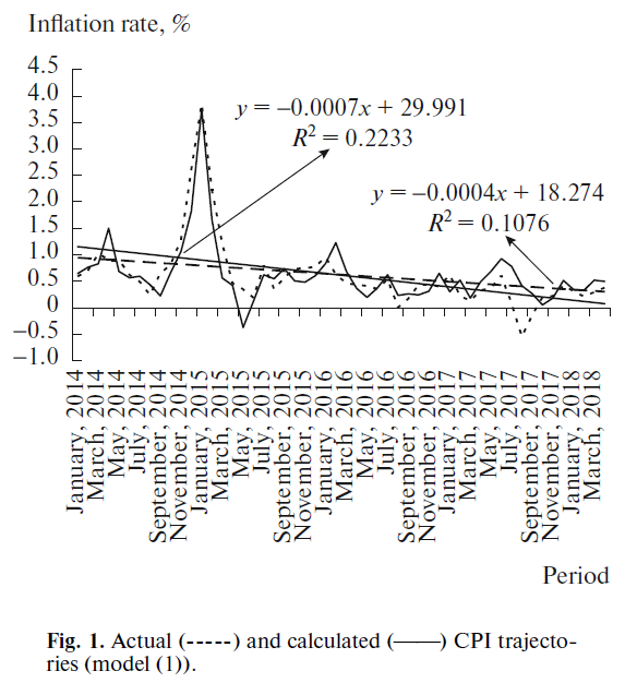
However, model (1) was constructed for inflation in the form of growth indices expressed as a percentage. This means that the CPI values in the model fluctuated around the 100–percent mark. However, in practice, inflation is estimated in growth rates that in monthly terms amount to fractions of a percent. In this regard, the extremely high accuracy in model (1) drops sharply in relation to the CPI indices–by two or three orders of magnitude–when moving to the rates of price growth. Thus, the computational experiment, suggesting a forecast for the constructed model for the known data for January–April 2018, enabled us to establish that the forecasting error by month in relation to the inflation index is 0.03; 0.12; 0.23, and 0.11%, while in relation to the inflation rates, its value is 10.7; 57.6; 80.3, and 31.1%, respectively; the last three values are unacceptably large. Thus, model (1), being theoretically and statistically acceptable, is not suitable for rolling applied forecasts.

This problem of data attribution is not unique in the construction of model (1). In order to identify the source of arising errors, let us consider the error related to the inflation rates according to model (1) accumulated in the course of one year (Table 3). Here, there are three interesting facts. The first: for the first two years, model (1) steadily understates the actual CPI values, while for the next two years it gives a steady overstatement of inflation. The second: in the fourth year, the forecasting error increases by an order in comparison with the third year. The third: the error over all four years is extremely small. These facts indicate that over the course of four years, there has been a change in the CPI formation regimes, each of which lasted for approximately two years. At the same time, model (1) aggregates these regimes and generally describes the process well; however, by the end of the period under consideration, the error begins to increase, indicating the loss of adequacy of the resulting econometric dependence over the specified time interval. The latter leads to the understanding that the applied purposes require the construction of the model on a shorter time interval covering the years of 2016–2017. In this case, there is a reason to assume that the model will reproduce the uniform mode of inflation suppression that was maintained by the Bank of Russia for the years indicated.

The computational experiments for the period of 2016–2017 gave the following alternative inflation model:

          (2)

N = 48; R² = 0.755; DW = 2.595; E = 0.26%,

where ΔW is the monthly financial and technological index of the ratio of labor productivity to wages; CSI is the consumer sentiment index; BCI is the business confidence index (among mining industry entrepreneurs); other indicators have not changed. Statistical characteristics of model (2) are satisfactory [2].

Comparison of models (1) and (2) shows that the policy of the Bank of Russia in 2016–2017 was drastically different from the measures of the previous biennium, which was reflected in the consistent and intensive suppression of inflation; this predetermined a completely different composition of markers in model (2) (see Table 1). In particular, the regime change was directed to the “washing out” of external factors and markers. Paradoxically, neither the exchange rate, nor the price for crude oil had a significant effect on domestic inflation in the period under review. In fact, it can be stated that the Bank of Russia has ensured that inflation in the country “became detached from” traditional external causes. At the same time, the key rate retained its value, although its influence “shifted” from one month in model (1) to three months in model (2). The change in the regulatory regime of the Bank of Russia has predetermined the limited length of retrospective series for model (2) (24 observations).

An important difference between models (1) and (2) is the composition of their regressors, namely, their number increased from four to five, and all of them belong to the group of internal ones. The nature of the markers has changed fundamentally; some of them started resembling complete factors of inflation. These include the financial and technological index ΔW, which shows the imbalance between technological changes in production (labor productivity) and financial costs (wage level). The emergence of mood parameters, both of consumers and producers, among the markers is also remarkable.

Another fundamental difference between models (1) and (2) is in the structure of explanatory factors. Thus, the calculations performed show that in model (1) the integral indicator of the influence of nonmonetary factors is 39.5%, whereas in model (2) it is 75.2% [3]. Thus, if in 2014–2015 the dominant part of the inflation process were monetary factors; then in 2016–2017, nonmonetary ones. In other words, even in recent years, the inflation phenomenon in Russia has undergone a fundamental transformation: in the initial period of international sanctions, it was formed mainly through monetary channels; and in a later period, at the expense of nonmonetary market forces.

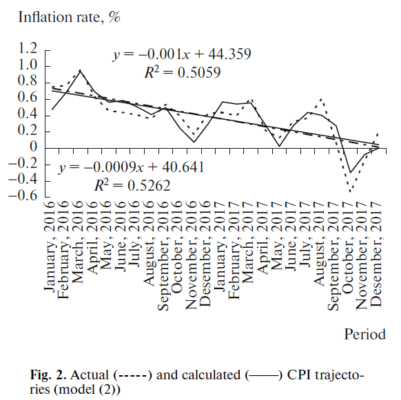
The accuracy of model (2) has significantly improved in comparison with model (1). So, the year error and the total error for two years, lie in the range of 5–6% (see Table 3), which can be considered a good result. At the same time, even within a shortened period, certain displacement of model estimates can be seen: if in the first year inflation is overestimated, in the second, it is underestimated. This is due to the slowing down of the Bank of Russia’s fight against inflation in 2017. However, in general, the accuracy of the model is such that the drawing of the actual and forecast CPI trajectories is almost the same, and their trends coincide almost completely (Fig. 2). In many ways, the improvement in the quality of model (2) in comparison with model (1) is associated with the rejection of the period with a powerful inflationary release in late 2014–early 2015 (Fig. 1).

Table 3. Distribution of the CPI approximation error accumulated over the year according to the models (1) and (2), %

The computational experiment related to the inflation projection by model (2) for three months in advance for the period from November 2017 to January 2018 has shown that the monthly inflation rate error was 28.8; 24.4, and 97.9%, respectively, which still goes beyond the permissible error limits. This fact indicates the impossibility of direct use of model (2) for the projection and predetermines further searches for ways to suppress errors for more accurate CPI prediction.

Calibration of the model with the use of a neural network. As seen above, the main problem of forecasting monthly inflation rates is their small value. It has already been pointed out in the literature that this problem is unsolvable within the framework of traditional econometric models [1]. There are various methods and techniques for “circumvention” of the problem. In our opinion, the construction of an “auxiliary” CPI forecasting model in the form of a neural network based on data from the existing econometric dependence (2) is the most preferred.

Four features of the inflation dynamics in Russia for the years under consideration can be identified. The first is almost complete coincidence of the actual and model trends (see Fig. 2); the second is the presence of strong fluctuations of actual CPI values around the trend, which requires the determination of the forecast range of inflation rates that should not be “overrun”; the third is the implicit cycling of CPI fluctuations around the trend line; and the fourth is the increase in the CPI fluctuation amplitude as their actual rates decrease. All these dynamic features of inflation can be taken into account through a well–trained neural network model.

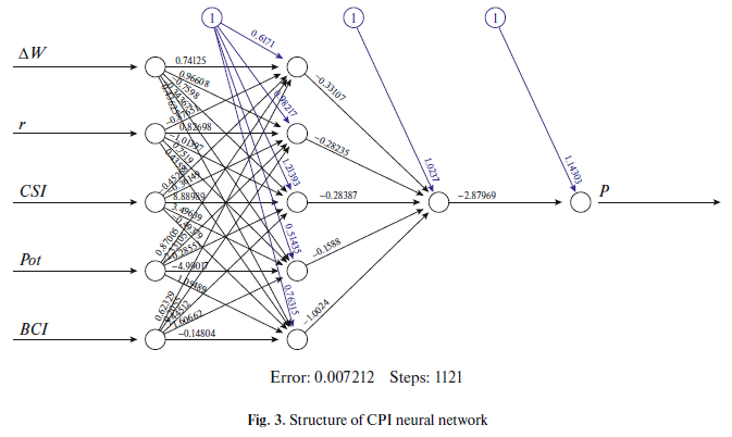
The construction of the applied neural network Web–Inf was performed in the RStudio software product (package Neuralnet) for a set of model variables (2). Five regressors of the econometric model were selected; therefore, only these variables were loaded into the Web–Inf model, which enabled us to calibrate forecast calculations as quickly and efficiently as possible.

The process of the network construction consisted of two successive stages. At the first stage, the network training was conducted on the basis of the main retrospective data (from February 2016 to October 2017) using the criterion of minimizing the sum of the squares of errors. This operation involved a random division of the sample into two parts without a chronological sequence: for training and for checking the accuracy. At the second stage, the test of adequacy of the trained network was conducted on test forecast data (the last three months of the retrospective series, from November 2017 to January 2018); with the criterion of minimizing the average absolute error of forecasts. Thus, a desired neural network must simultaneously meet two requirements, i.e., to show a low error in regard to the test data and to show a low error in regard to the forecast data. As a result, in the selection process, hundreds of thousands of neural networks that met the training criterion but showed unsatisfactory results in relation to the forecast sampling, were rejected.

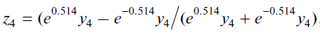
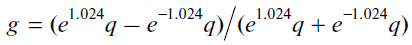
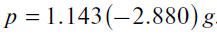
For a better understanding of the calibration algorithm of a desired dependence, let us “decipher” the neural network constructed in Fig. 3:

     (3)

    (4)

     (5)

    (6)

   (7)

                                     (8)

                              (9)

                                   (10)

                                  (11)

                                 (12)

         (13)

                                          (14)

                                                                                 (15)

It should be noted that the approach used in the study is not widespread, since the prediction accuracy is usually considered the main attribute of the quality of a neural network. In this case, the traditional approach was strengthened by adding two filters of accuracy: the main filter (on the basis of retrospective data) and an additional one (on the basis of test forecast data). All the data of the model Web–Inf were preliminarily normalized according to the standard formula X_norm=(Х–X_min)/(X_max–X_min). The minimum average error of prediction of normalized values (0.5%) was achieved with an error on the test sampling (0.7%) under the following conditions: two hidden layers of five and one neuron, respectively (Fig. 3); 1121 network training steps; the activation function is a hyperbolic tangent; the error function is the sum of squared errors; and the activation function is excluded in the transition to the output layer of neurons. The remaining parameters had a minor effect on the training process.

The risk of undertraining of the neural network is almost excluded for the constructed neural network model due to the small number of input variables (five indicators). In order to avoid overtraining, the authors used the abovementioned double accuracy filter.

In order to assess the efficiency of the use of the Web–Inf model, it is necessary to compare the quality of test predictions of inflation rates obtained on the basis of the econometric model (2) and the Web–Inf model. As can be seen from Table 4, the preference of the neural network with respect to the criterion of forecast accuracy is overwhelming. Thus, the second step in constructing the inflation model by calibrating the “primary” econometric dependence (2) by means of the “secondary” neural–network model has fully justified itself.

Table 4. Test forecasts of inflation rate according to the models (2) and Web–Inf

It should be stressed that comparing the accuracy of predictions according to two models is intended to show not the prognostic potential of the neural network itself, but its ability to improve the predictive properties of the primary econometric model (2). At the same time, good statistical parameters of the regression model (2), as a rule, guarantee highly accurate forecasts on the base of the Web–Inf model, while in relation to the neural network models constructed in automatic mode (without preliminary selection of explanatory variables using model (2)), there is no such guarantee due to the risk of their overtraining.

Since the two–step forecasting procedure is a sequential combination of econometric and neural network models, the authors will designate the desired hybrid model as Eco–Web.

* * *

Complication of the inflation phenomenon in recent decades and its presentation in the form of a nonfixed set of combinations of a large number of variables of different nature has led to the fact that its prediction with the use of traditional models does not justify itself. The way out of this situation is seen in the use of a more complex prediction algorithm, based on the hybrid model that represents a combination of econometric and neural network tools. Such a computational complex has greater flexibility in relation to the short-term fluctuations; at the same time it remains relatively simple. The testing of the hybrid model Eco–Web has shown its efficiency for short (two or three months) forecast horizons; however, the attempts to extend the forecast period for several months do not give positive results. Thus, even hybrid models have strictly limited predictive capabilities.

At the same time, the practice of applying hybrid models suggests development in various directions. For example, the primary selection of significant variables can be performed not on the basis of a CPI correlation matrix, but with the use of a primary neural network model. Thus, the “econometric model–neural network” scheme used in this work can be transformed into a more complex chain, i.e., “neural network–econometric model–neural network”. It is possible to supplement the hybrid model with an analytical interface aimed at identifying threshold events that signal the need to revise the set of explanatory variables and the model specification [2]. Apparently, the adequacy of model inflation forecasts can only be ensured by further complicating the entire analytical construction of applied calculations.

This work was prepared on the basis of the study “Technological, Structural, and Social Factors of Long–Term Economic Growth” supported by the Financial University under the Government of the Russian Federation financed from the budget (АААА-А19-119080990043-0).

References

1. E.V. Balatskii and M.A. Yurevich, “Using neural networks to predict inflation: New opportunities,” Vestn. Ural. Fed. Univ., Ser.: Ekon. 17 (5), 823–838 (2018). https://doi.org/10.15826/vestnik.2018.17.5.037

2. E.V. Balatskii and N.A. Ekimova, “Accounting for threshold non–monetary events in hybrid inflation models,” Vopr. Regul. Ekon. 10 (1), 6–24 (2019). https://doi.org/10.17835/2078-5429.2019.10.1.006-024

3. J.M. Bates and C.W.J. Granger, “The combination of forecasts,” J. Oper. Res. Soc. 20 (4), 451–468 (1969).

4. P. Newbold and C.W.J. Granger, “Experience with forecasting univariate time series and combination of forecasts,” J. R. Stat. Soc. 137 (2), 131–164 (1974).

5. E.V. Balatskii and M.A. Yurevich, “Inflation forecasting: The practice of using synthetic procedures,” Mir Nov. Ekon. 12 (4), 20–31 (2018).

6. A.A. Vasil’ev, “Genesis of hybrid forecasting models based on the combination of predictions,” Vestn. Tver. Gos. Univ., Ser.: Ekon. Upr., No. 1, 316–331 (2014).

7. P.G. Zhang, “Time series forecasting using a hybrid ARIMA and neural network model,” Neurocomputing 50 (17), 159–175 (2003).

8. F.P. Tian and L.L. Ma, “Forecast of cerebral infraction incidence rate based on BP Neural Network and ARIMA Combined Model,” in International Symposium on Intelligence Information Processing and Trusted Computing (2010), pp. 216–219. https://doi.org/10.1109/iptc.2010.7

9. B. Wang, W.N. Hao, G. Chen, D.C. He, and B.A. Feng, “Wavelet neural network forecasting model based on ARIMA,” Appl. Mech. Mater. 347–350, 3013–3018 (2013).

https://doi.org/10.1371/journal.pone.0175915

10. O.O. Bozkurt, G. Biricik, and Z.C. Taysi, “Artificial neural network and SARIMA based models for power load forecasting in Turkish electricity market,” PLOS ONE, No. 12 (2017). https://doi.org/10.1371/journal.pone.0175915

11. L.A. Xuemei, D. Lixing, S. Ming, X. Gang, and L. Jibin, “Novel air–conditioning load prediction based on ARIMA and BPNN model,” in Asia–Pacific Conference on Information Processing (2009). https://doi.org/10.1109/apcip.2009.21

12. S.R. Moiseev, “The rules of monetary policy,” Finansy Kredit, No. 16, 37–46 (2002).

13. N.A. Ekimova, “Institutional risks: In search for inflation determinants,” Vestn. Ural. Fed. Univ., Ser.: Ekon. Upr. 17 (5), 732–750 (2018).

14. V. Hnatkovskay, A. Lahiriy, and C. Veghz, The Exchange Rate Response Puzzle (2012). https://ss-rn.com/abstract=1996693.

15. J. Cochrane, Do Higher Interest Rates Raise or Lower Inflation? (2016). https://www.newyorkfed.org/medi-alibrary/media/research/conference/2016/woodford/ cochrane_dohigherinterestratesraiseorlowerinflation.

16. J. Cochrane, The Grumpy Economist (2015). https://johnhcochrane.blogspot.com/2015/11/early-fisherism.html.

17. T. Gorshkova and E. Sinel’nikova, “Comparative analysis of the predictive properties of Russia’s inflation models,” Nauchn. Vestn. Inst. Ekon. Polit. im. Gaidara, No. 6, 34–41 (2016).