Introduction to the problem

The period since the start of economic reform has not led to the balancing of the Russian economy. So far, the great majority of Russian economic markets feature excess demand, resulting in exorbitant prices of goods and services. This emphasizes the issue of unwarranted overpricing against the background of a small–capacity market. The immediate cause is the virtual lack of competition mechanisms in Russia. In this connection it would be appropriate to recall H. Ford’s recommendations for pay raising and price cutting [1–2]. He saw the keystone of success and main instrument of this policy in cost reduction and, accordingly, manufacturers' efforts to find new ways of reducing costs. An antithetical concept is at work in Russia: manufacturers are anxious to keep the prices of their products up without any shifts in their manufacturing technologies or serious loss to their business. Obviously, if this trend persists, the quality and quantity characteristics of many economic markets in Russia may be destroyed.

The situation is aggravated by an unfavorable institutional climate, although it has long been clear on the intuitive level that the costs incurred by economic agents in maintaining a normal institutional environment and infrastructure are out of line with what they are getting in return. In other words, the price of the institutional benefits that economic agents pay as taxes to the government does not match the quality and quantity of the services provided by the government. This imbalance of the institutional benefits market has a negative effect on general economic equilibrium and adds to the distortion of equilibrium prices.

The problem of distortion of equilibrium prices on the macrofactor market has been discussed elsewhere [3–5]. Yet, some new problems have since become visible, which call for a systemic explanation.

First, it is still unclear how two important theoretical constructs are related: the equilibrium price distortion equation (see [5]) and Walras’ law. On examination the two constructs reveal obvious similarities, yet their deeper linkage is still elusive. Establishing their relation is very important for two reasons. On the one hand, all the elements of the equilibrium price distortion equation are quantifiable, whereas this is not true of Walras’ law. On the other, Walras’ law makes it possible to move from the study of nonequilibrium prices to a meaningful analysis of economic markets. Thus, aligning the equilibrium price distortion equation and Walras’ law is a pressing methodological need.

Second, it is not clear how the institutional factor can be incorporated in the general economic equilibrium framework. Walras’ law in its conventional form does not provide for such synthesis. On the other hand, the plain fact is that the institutional factor is at least as important as traditional factors such as labor and capital. Like any economic resource, institutional benefits have equilibrium prices of their own, which in the course of economic activity may be distorted, thereby introducing noticeable changes in the equilibrium price structure. Therefore, building a more general, integral model of economic equilibrium, which incorporates the institutional factor, is an important theoretical challenge.

Third, as the theory uses such notions as equilibrium prices and economic market flexibility it demands that more empiric data be accumulated. Drawing upon additional statistical data reflecting the state of different economies would create a more solid base for further theoretical constructs. Thus, expanding the geography of applied research is an integral element of in–depth study of economic equilibrium problems.

Fourth, thorough macroeconomic diagnosis assumes some understanding of the potential of economic markets, in particular, the labor market. To achieve it, we should proceed from the notion of a “natural” (normal) rate of unemployment, which is proper to an economy at a certain stage of development. The notions of equilibrium prices at macrofactor markets and the variance of actual prices help determine the level of equilibrium margin that can be achieved by a particular labor market. However, in some cases solving this problem involves “nonlinear” computations. We need to accumulate some positive experience of diagnosing national labor markets using equilibrium theory techniques in order to ascertain some procedural subtleties in the macroeconomic diagnostics application tools.

Two–factor model of economic equilibrium

We shall derive an equilibrium price distortion equation in a reduced form (for details, see [5]). Consider the net income X derived from production and consisting of the wage bill and the mass of clean profit: X = π + WL, where L is employment volume, W is the average annual wages of wage earners, π is the mass of clean profit gained by the businessman after taxes. This equation can be rewritten in a more operational form:

X= WL + rI                                                                                                                                                                                   (1)

where I is fixed investment, r = π/I is average annual rate of return per unit investment.

Thus, net income is calculated by formula (1), where all the four variables (L, W, I, π) are initial statistical aggregates involved at both micro– and macrolevels, with W and r used as the actual prices of labor and capital.

To determine the equilibrium prices of labor and capital we assume that the relation of net income X to macrofactors is described by a homogeneous production function of the degree of homogeneity ν; X=X(L, I).

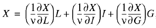
Then, the following Euler expansion is valid [1]:

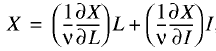                                                                                  (2)

where W*=(1/v)(dX/dL) is equilibrium wage (equilibrium price of labor) and r*=(1/v)(∂X/∂I) is equilibrium rate of return (equilibrium price of capital). It is readily apparent that, with this interpretation, the equilibrium prices of factors are determined by their marginal productivity, and hence, they match the actual production contribution of each factor to X generation.

Formula (2) show the generation of net income according to the mass and effectiveness of macrofactors, and formula (1), the spending of net income on the compensation of macrofactors according to their mass and actual prices. By joining (1) and (2) we arrive at a fundamental equation for equilibrium price distortion at labor and capital markets:

(W* – W)L + (r* – r)I = 0.                                                                                                                                                            (3)

In accordance with equation (3) in the macrofactor market in general, there is always a price equilibrium: if a factor’s services are underpaid on one market, they are overpaid on another market. In other words, if the actual price of one factor is understated, that of another is automatically overstated.

Assuming that aggregate demand and aggregate supply are in equilibrium on the commodity market, Walras’ law for a macroeconomic system can be written as

(L* – L)W + (I* – I)r = 0                                                                                                                                                              (4)

where L* is labor demand, I* is fixed investment demand, L is labor supply, and I fixed investment supply [2].

Expression (4) means that there is always global equilibrium in the system: if there is excess demand on one market, there is excess supply on another. For example, if unemployment is on the rise in a country, the public will necessarily suffer from underinvestment.

A comparison of (3) and (4) reveals their striking similarity. For instance, equation (4) recognizes volumetric market imbalances weighted according to actual prices, whereas equation (3) deals with price distortions on markets weighted by actual volumes of macrofactors. Although they reflect different aspects of operation of macroeconomic markets and were derived on quite different theoretical premises and assumptions, their similarity is too obvious to be accidental.

Let us concentrate on the relationship of equations (3) and (4). We shall find out whether it is possible to reduce them to some third theoretical construct. It will help us understand how equilibrium price distortions on markets are related to deviations of demand from supply.

Equivalence conditions of the equilibrium price distortion equation and Walras’ law

For analytical purposes the distortion of equilibrium prices can be more conveniently appraised in relative terms. To this effect equation (3) must be rewritten to take into account the structural parameter reflecting the share of the wage bill in net income λ = WL/X:

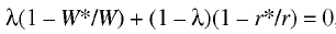   (5)

where W*/W is equilibrium wage distortion factor, r*/r is rate of return on capital distortion factor. These price distortion factors are weighted according to the contribution of respective factors to total net income.

Further analysis involves a hypothesis according to which price distortion on factor markets affects the markets themselves, including the demand and supply aggregates. Then, the relationship between for market characteristics–demand, supply, actual price, and equilibrium price–is given by the following relation [4–5]:

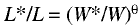                                                                                                 (6)

where θ is a parameter characterizing labor market flexibility, i.e., the mutual adaptability of the demand – supply and equilibrium price – actual price ratios. In other words, the parameter of labor market flexibility reflects the degree of reciprocity of the two kinds of market disequilibrium: price and volume.

A similar model can be written for the capital market:

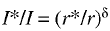                                                                                                       (7)

where δ is a parameter characterizing the flexibility of the capital market. [3]

Thus, the meaning of models (6) and (7) is that they help introduce in our analysis the notions of market flexibility, which is of both theoretical and applied relevance.

For ease of further constructs we rewrite Walras’ law (4) in a form that includes relative characteristics of market equilibrium distortion:

                             (8)

where λ*=WL/X and λ**=rI/X. Unlike λ, λ* recognizes labor supply rather than employment volume, which in most cases equals labor demand. Thus, the weight coefficients in equations (5) and (8) are, generally, different. In Walras’ law, one weight is always greater than its counterpart in equation (5).

Inserting formulas (6) and (7) in relation (5) we arrive at a price distortion equation of the form

(9)

A comparison of (8) and (9) will provide an answer to the foregoing question about the nature of the relationship between equilibrium price distortion and Walras’ law: if factor markets have absolute flexibility, i.e., θ = δ = 1, then the equilibrium price distortion equation and Walras’ law are identical to an accuracy of weight coefficients; absolute identity is unattainable. The ideal flexibility of markets is the equivalence condition of the two theoretical constructs under consideration. [4] This results entitles us to draw two important methodological conclusions.

First, the equilibrium price distortion equation as a theoretical construct is preferable to Walras’ law as it incorporates Walras’ law as a special case and, besides, assumes quantitative measurements. To elucidate, Walras’ law is not, as a rule, liable to verification because it incorporates the quantity of demand, which largely defies measurement. It can be determined indirectly in the case of labor market but not capital market. At least, it would involve solving independent methodological and measurement problems.

Second, Walras’ law in its classical form has a significant theoretical deficiency, namely, failure to recognize the effect of economic market flexibility. In point of fact, Walras’ law presupposes that all markets under consideration perform perfectly and are, hence, perfectly flexible. In reality, economic markets are more prone to dormancy, stagnancy, and inertia. Moreover, in the absence of proper market flexibility all kinds of anomalous effects are bound to arise, which are currently in the focus of attention of economic theorists (see, e.g., [9]).

Therefore, the revealed formal similarity of the equivalent price distortion equation (3) and Walras’ law (4) is not spurious and superficial but reflect the organic unity of their two underlying methodologies. Yet, it would be wrong to speak of the full equality and ideal congruence of the two equations as they are in a state of rather rigid methodological subordination. In some ideal case, when the price and volumetric characteristics of economic markets are fully balanced, the differences between the two methodologies and equations all but disappear. In practice, however, this is a rather rare occurrence.

Three–factor economic equilibrium model; embedding the institutional factor into equilibrium theory

As shown by the practice of applied calculations, a two–factor model of equilibrium price distortion quite adequately describes real–life processes [5]. However, modem theory calls for the extension of the model, i.e., the incorporation of the institutional factor. Besides, the statistical index of net income used in the two–factor model is too narrow and should be expanded so as to go over to the value added index.

In view of the need for theoretical extension of the model, we shall generalize the equilibrium concepts by introducing, in addition to the labor and capital markets, a third one, the institutional market. In this case, the income X derived from production will be the sum of the wage bill, profit margin, and tax payments: X=T+rI+WL, where T is the sum of all taxes paid by the producer. This method of income calculation assumes that income is shared between three groups of economic agents: employers (capital), wage earners (labor), and government (institutions). The government, which withdraws part of the value added as taxes, does not do it as simple fiscal withdrawal; by means of taxes it receives a price for its “work” of ensuring the normal functioning of the whole system of institutions and social infrastructure. It is for its efforts to maintain the institutional environment in a normal state that business shares with it some of its income. In this process, the institutional factor in the form of formal (normative–legal) and informal (moral) norms supporting the business community, acts as a fully–fledged factor of production. Without a normal institutional environment fully–fledged economic operations are very difficult if not impossible.

All the points we made seem to be quite natural, and difficulties appear mainly when we set out to account for and measure the institutional factor. What are possible approaches to this problem?

To begin with, we should proceed from the premise that there is no point in measuring the government’s institutional contribution by common quantitative indices. Indeed, the mere number of institutions give no indication of the institutional environment itself. Therefore, we feel that it is advisable to measure the quality of the institutional environment. Since it is always in place, what really matters is not its quantitative characteristics but qualitative ones. An increase or decrease in taxes always implicitly assumes an increase or decrease in the quality of institutional support.

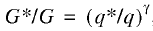
Relying on these ideas we introduce a quality indicator G of institutional environment. The observed quality G of institutional environment is secured by the taxes T, which enables one to measure the actual price q of some quality unit: q=T/G. Of course, the price expression depends on the chosen quality scale of institutional support. Then, the shared earned income is described by the dependence

X = WL + rI+ qG                                                                                                                                                                        (10)

We note that in this case the aggregate X is an index very similar to value added. It differs from the conventional index of value added by the quantity of amortization. Consequently, the three–factor model is much more exact in describing the real process of new value creation.

We further presuppose that X is linked to the three facts by the homogeneous production–institutional function of degree of homogeneity ν: X=X(L, I, G). Then, the three–factor Euler expansion is good:

                        (11)

where W*=(1/v)(∂X/∂L) is the equilibrium price of labor, r*=(1/ν)(∂X/∂I) is the equilibrium price of capital, and q*=(1/ν)(∂X/∂G) is the equilibrium price of institutions. Relation (11) describes income creation under the action of three factors and relation (11), its expenditure on paying for these factors. By aligning formulas (10) and (11) we arrive at a three–factor equation of equilibrium price distortion:

(W*–W)L + (r* – r)I + (q* – q)G = 0                                                                                                                                           (12)

To switch to relative measures we rewrite equation (12) as follows:

                                           (13)

where λ=WL/X is the share of the wage bill in value added X; ζ=T/X is the share of taxes in the income X; μ=π/X is the share of clean profit in X; μ=1–λ–ζ.

Equation (13) features relative price distortions weighted by share factor coefficients. The resulting theoretical construct has at least two distinguishing characteristics.

First, the quantity of tax burden appears as a price distortion multiplier on the institutional services market. This follows directly from the fact that the share indicator ζ acts as a relative value of the tax burden. Correspondingly, given distortions of the equilibrium prices of institutions benefits, any increase in the tax burden results in a greater total disequilibrium potential of the economic system. In the absence of equilibrium price distortions, tax burden growth does not by itself act as a source of economic deformation. In other words, the tax factor is only activated with the appearance of disparities between actual and equilibrium prices of market institutions.

Second, the three–factor price equilibrium model assumes a very complicated mechanism of income redistribution. In contrast to the two factor “labor–capital” alternative in equation (13), there are three economic agents: capital (employer capitalist), labor (wage earners), and government (officialdom). Accordingly, labor underpayment may be accompanied by underpayment of capital’s contribution against the background of the government’s acquisition of an unjustifiably large portion of value added; the two–factor equilibrium model does not envisage this outcome. In addition to the above situation, there may appear other complex combinations involving unjustified acquisition of value added.

The notion of flexibility also applies to the institutional market; it is formalized by means of this model:

                                                                               (14)

where G* is requisite quality of the institutional environment (institutional quality demand); G is actually observable quality of the institutional environment (institutional quality supply), and γ is a parameter describing the flexibility of the institutional market.

By inserting models (6), (7), and (14) in equation (13) we arrive at a generalized Walras’ law:

                                          (15)

Presented in this form, the equilibrium price distortion equation shows that a system’s balance may be upset by a mismatch not only of demand and supply at labor and capital markets but also the actual and required quality of institutional support to business. Therefore, a single theoretical construct joins together qualitative and quantitative characteristics of dissimilar economic markets. Also, the institutional factor is incorporated in Walras’ law, which is not recognized in conventional Walras equations. Furthermore, the absence of the institutional factor is believed to be one of the deficiencies of Walras’ law. Equation (15) remedies this deficiency.

Let us revert to the measurement of institutional quality G. Presently, it does not seem possible to suggest a rational method of objective appraisal of institutional environment. We should likely make use of a somewhat different methodology, which has been increasingly applied in macroeconomic diagnostics of late. These are, as a rule, evaluation procedures relying on sampling surveys. One applicable variety of this approach is a survey of businessmen’s degree of satisfaction with the quality of their institutional environment. Despite certain variability in computing the parameter of institutional quality, the possibility of obtaining meaning numeric estimates in this sphere is beyond question. Building institutional indicators is an increasingly common practice, so computation problems cannot be a serious impediment to the application of a generalized three–factor scheme of economic equilibrium.

Econometric estimation of the distortion of equilibrium prices at the labor market

To fully reveal the possible effectiveness of the equilibrium price distortion equation we make a series of applied calculations for three countries, the United States, Britain, and Russia, relying on two–factor equilibrium model (5).

Since price distortions at labor and capital markets are inversely related we shall limit ourselves to analyzing price distortions at the labor market. To this end we shall consider the values of the relative distortion factor of the equilibrium wage ε=W*/W–1.

For the United States economy 1987–2000 we built a Cobb–Douglas production function as the following econometric relationship: [5]

                                                          (16)

N = 14; R² = 0.988; F = 454.14; DW = 1.06.

Regression coefficients (16) have underneath them their standard errors in parentheses and their t–statistics in square brackets; N is number of observations; R² is coefficient of determination; F is the value of F–statistics; DW is Durbin–Watson coefficient of autocorrelation; a similar notation system is used in what follows.

Relation (16) passes all tests, including the t–statistics of coefficients of regression at a 90% significance level. Consequently, model (16) is effective and can be used in further applied calculations of equilibrium parameters of the system.

A peculiarity of econometric model (16) is that instead of a fixed investment index (I) it uses fixed capital (K) itself. This replacement is perfectly acceptable and it does not lead to any substantive and methodological adjustments in the original scheme. Calculations of price characteristics of the US labor market by model (16), listed in Table 1, shows that the distortion factor of the price of labor is a negative quantity. It means that labor is clearly overpaid to the prejudice of capital investment. [6]

Table 1. Price characteristics of the US labor market 1987–2000

We could also build a production function for the British economy 1979–2005:

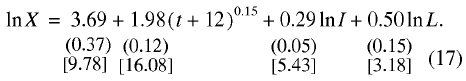                                (17)

N= 24; R² = 0.989; F = 655.35; DW = 1.40.

Its distinctive feature is the inclusion, in addition to two principal factors of production, of a trend component [7]. This modification of the basic relationship does not interfere with the modeling conditions or lead to errors. Taking into account basic statistical tests, econometric relation (17) can, on the whole, be accepted as workable [8].

Table 2 lists estimated equilibrium values of the British economy, based on model (17), which show that the British and American labor markets had much in common. In particular, wages in both countries exceeded the equilibrium value. However, according to our calculations, disequilibrium was somewhat smaller in the United States than in Britain. The averaged value of the distortion coefficient of the price of labor in the United States was 26% compared to 33% in Britain. Thus, the US economy was somewhat better balanced than the British and was closer to the perfect (equilibrium) state. Most important, the US and British economies are functioning on the principle of overpayment of hired labor.

Table 2. Price characteristics of the British labor market 1979–2002

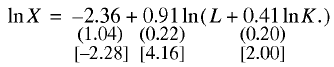
The Russian economy is a fundamental alternative to the United States and Britain. We built for it the following econometric relation for 1989–2002:

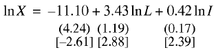        (18)

N= 13; R² = 0.964; F= 136.52; DW= 2.74.

Model (18) successfully passes all the statistical tests, including the t–statistics of regression coefficients at a 95% significance level. Thus, it is quite operable and can be used in further applied calculations, listed in Table 3, which help ascertain two important facts.

Table 3. Price characteristics of the Russian labor market 1990–2002

First, the rate of labor exploitation in Russia is positive and averages 24%. It means that labor is steadily underpaid by about a quarter. The beneficiary is capital, whose rate of return is systematically inflated. Second, the economic model that evolved in Russia was notable for a high degree of disequilibrium (the distortion coefficient of the price of labor was as high as 50% in 1999) and instability (the distortion factor fluctuated within (–6.3%) to (+50.7%)).

Therefore, two characteristics distinguish the Russian economy from the American and British. By the characteristic of deviation from equilibrium the American and British economies belong to the class of countries featuring hidden “subsidizing” of hired labor by capital, whereas the Russian economy belongs to the class of countries with a high level of exploitation of hired labor. By the characteristic of stability of the established mode of operation the American and British economies belong to the class of countries characterized by high stability in growth, whereas Russia belong to the class of transition economies, characterized by constant fluctuations around equilibrium state.

Price distortion and economic market stability

Our calculation of price distortion at macrofactor markets are of great methodological importance for better understanding key functional properties of different economies. The fact is that the direction of deviation of actual prices from their equilibrium values has not only social but also purely economic implications. Let us examine this aspect of the problem in more detail. [9]

An economic regime where the actual price of labor exceed the equilibrium price (W > W*) means the following mechanism of conjugation of the labor and capital markets: the overpayment of labor and the downward bias of rate of return stimulates the market demand for goods and services; high solvent demand makes it easier for producers to sell their products, thereby assisting them to receive a suitable rate of return; part of the rate of return received by producers is given back to wage earners, which leads to another overpayment of labor and a new rise in solvent demand, etc. The perpetual repetition of this cycle maintains the economic system in homeostasis. In practice, the following process takes place. To create a financial base for their business producers share their earnings with hired labor. At the next capital cycle, the money surplus received by hired labor is expended on production process maintenance. Hence, this regime is perfectly natural and economic systems operating in this mode are likely to be stable in consequence of the cancellation effect between feedback and feedforward. Their action can be roughly described as follows: if the equilibrium price of labor is set too high, then, all other conditions being equal, it will lead to a rise in the producer’s rate of return, and the rate of return is reduced on account of an increased equilibrium price of labor. This gives rise to a self-regulating process of reproduction of capital, and the national economy is functioning in a stable homeostasis.

A functional regime in which the actual price of labor is below the equilibrium one (W < W*) generates an entirely different mechanism of conjugation of labor and capital markets: the underpayment of labor and the upward bias of rate of return undercut the market demand for goods and services; low solvent demand impedes the sales of goods thereby complicating the receipt of proper rate of return; producers augment the rate of profit received by once again underpaying their labor, which undercuts solvent demand still more, etc. The infinite repetition of this cycle draws the economic system nearer to depression and recession. In that case, the following process takes place: by appropriating part of the common income producers undermine the financial basis of their business. The surplus money received by producers increases at the next turn of the circulation of capital, which tends to enhance income differences among the population. Therefore, the regime in question is unnatural and economic systems functioning in this regime are likely to be unstable on account of the enhancement effect between feedforward and feedback. Here, the action of feedforward and feedback is as follows: an underestimated equilibrium price of labor, all other conditions being equal, leads to a fall of the producer’s rate of return, and the fall of the producer' rate of return stimulated another underestimation of the equilibrium price of labor. This results in a self–induced process of economic collapse, with the national economy gravitating to recession.

On this evidence it is easy to see which of the two regimes of equilibrium price distortion is to be preferred. In this case we observe that countries of traditional capitalism, such as Britain and the United States, abide by the “homeostatic” regime of disequilibrium price formation, while Russia sticks to an unstable “depressive” regime. This fact provides a new perspective on the sustainability of the Western model of capi­talism and helps in understanding the kind of problems that “neocapitalist” countries like Russia are going to face in the future.

Estimating the flexibility of national labor markets; the role of the parameter of market flexibility in producing anomalous effects

The notion of flexibility of economic markets we introduced as a characteristic of “friction” is of tremendous theoretical and practical value. In order to verify and “digitize” this notion we shall calculate the labor market flexibility for the US, British, and Russian economies.

Using basic model (6) and the notation L*/L = Ω = l – ω, where Ω is rate of employment, ω is rate of unemployment, it is easy to calculate the parameter of market flexibility. The results of applied calculations for the US economy are listed in Table 4, for Britain, in Table 5, and for Russia, in Table 6. [10]

Table 4. Characteristics of the US labor market 1987–2000

Table 5. Characteristics of the British labor market 1979–2002

Table 6. Characteristics of the Russian labor market 1990–2002

These figures lead to several conclusions.

First, the response of the Russian labor market to price distortions is anomalous compared to the American and British markets. This is demonstrated by the negative sign of θ for the Russian economy and the positive sign for the US and British economies. [11] The negative sign points to an essentially abnormal response of the national labor market to equilibrium wage distortion. The logic of the market and that of model (6) suggests that unemployment arise when the price of labor is higher than the equilibrium value (the case of the United States and Britain). If labor is underpaid, the system must, on the contrary, generate excess labor demand, or overemployment. It was the case in the former Soviet Union [3] and a similar situation should have prevailed in today’s Russia, but it never happened this way. It appears that transition economies like Russia suffer from two afflictions of capitalism at once, labor exploitation and unemployment.

Second, the United States greatly surpasses Britain in the absolute value of labor market flexibility: an average of 0.19 against 0.15. Thus, the US market is more flexible than the British one.

Third, the Russian labor market is less predictable than the American, which is, in turn, less predictable than the British one. This fact follows from an analysis of the dynamic behavior of the quantity θ. It varies within the range 0.132 to 0.237 for the United States, within 0.118 to 0.180 for Britain, and [–1.611] to 3.109 for Russia. Accordingly, the fluctuation band is 0.062 units for Britain, 0.105 for the United States, and 4.720 for Russia. What it means is that in Britain and the United States, labor market flexibility is an independent and stable factor of the economic mechanism, whereas in Russia, this property of the labor market is only evolving and it has not yet taken final shape as an independent economic phenomenon.

The parameter of labor market flexibility in addition to a diagnostic function performs an explanatory function. The point is that anomalous phenomena on the Russian labor market can be explained by the immaturity and inefficiency of the market as such. Furthermore, the estimates in Table 6 suggest that the labor market in Russia has not yet fully emerged and, hence, it cannot regulate key macroeconomic ratios. In other words, market mechanisms cannot function normally as they have not yet formed as such. This largely explains some odd phenomena on the Russian labor market.

“Natural” level of unemployment: differences in configuration between national labor markets

The concept of disequilibrium prices of macrofactors among other things serves as a framework for determining such an important quantity as “natural (normal) rate of unemployment.” To this end we must merely relate the rate of employment/unemployment Ω(ω) and the coefficient of distortion of the equilibrium price of labor W*/W. It turns out that this relationship exists for all the economies under review–the United States, Britain, and Russia.

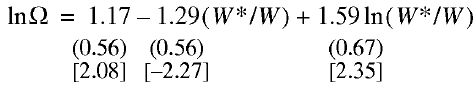
Calculations for the US economy 1987–2000 established the following econometric relationship:

                        (19)

N= 14; R² = 0.554; F = 6.83; DW = 0.82.

Regression relationship (13) successfully passes all tests, including t–statistics of the regression coefficients at a 90% significance level and can be used in future analyses of the US national labor market. Therefore, there is a stable relationship between the employment rate indicators and the equilibrium price distortion coefficient.

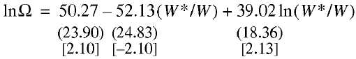
Similar calculations for the Russian economy 1992–2002 led to the following econometric relationship (early years of the original statistical series were rejected because they created hindrances to model calibration):

                                (20)

N= 11; R² = 0.456; F= 3.35; DW= 0.74.

Regression relationship (14), too, successfully passes all tests, including t–statistics of the regression coefficients at a 90% significance level.

For the British economy 1983–1995, a more sophisticated econometric relationship was built:

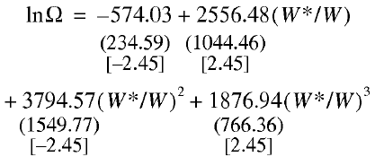                                      (21)

N= 13; R² = 0.437; F = 2.33; DW =2.21.

This model is quite satisfactory and can be used in further calculations.

Econometric models (19)–(21) make it possible not only to predict employment rate depending on the price situation on the labor market but also to determine the “natural” or “normal” rate of unemployment. To this end calculations are made by the following algorithm.

I. The relationship Ω = Ω(u), where u = W*/W, defined by functions (19)–(21), is nonlinear. For this relationship find the maximum point for the price distortion index u_max for dΩ/du = 0.

II. For the point u_max there is a corresponding maximum employment point Ω_max = Ω(u_max), which is automatically calculated by inserting the value of u_max in the available relationships.

III. The point Ω_max does not, as a rule, coincide with unity, hence, full employment proves to be unattainable. Then, the disparity between full employment and maximum employment will reflect the rate of “natural” unemployment ω_NAT, calculated by the formula: ω_NAT = 1 – Ω_max.

Calculations based on model (19) show that for the United States, u_max = 0.75, to which there correspond maximum employment Ω_max = 0.95. Accordingly, the “natural” rate of unemployment for the United States is ω_NAT = 5%. For Russia similar calculations by model (20) produce the value of the point u_max = 1.23, to which there corresponds peak employments Ω_max = 0.92. Hence, the “natural” rate of unemployment for Russia is ω_NOR =8%, which is 3 percentage points higher than in the United States.

Data for Britain require a somewhat more complex analysis. In accordance with model (21) the curve Ω = Ω(u) has the maximum point Ω_max = 0.95 at u_max = 0.66 and the minimum point Ω_max = 0.94 at u_max = 0.69. Given that the actual values of the distortion coefficient of the price of labor for Britain were within the interval where critical points are found, it would be safe to say that the “natural” rate of unemployment for that country is ω_NOR = 5%, which is the same as in the United States. If the price distortion at the British labor market decreases below 30%, full employment is entirely possible.

These findings demonstrate some contradiction between the price equilibrium at the factor market and the condition of the relevant markets. It follows from the fact that the labor market finds itself in the best shape by no means at the perfect equilibrium of factor prices. While overpayment of hired labor is “useful” for the US and British labor markets, in the case of the Russian labor market underpayment is more beneficial. Thus, the markets under review formed quite differently and function in entirely different economic modes. Correspondingly, any attempt to translate economic formulas of advanced Western countries to transition economies is prone to error. As indicated before, these discrepancies and anomalies are rooted in the different flexibilities of national labor markets.

References

1. Henry Ford, My Life and Work (Popurri, Minsk, 2004) [translated from English].

2. Henry Ford, Today and Tomorrow (ID “Ural Yur Izdat”, Yekaterinburg, 2004) [translated from English].

3. E. V. Balatskii, “Value Imbalances in the Labor Market,” Ekon. Mat. Metody, No. 1 (1993).

4. E. V. Balatskii, “Labor Market Flexibility: A Macroeconomic Estimation,” Mirovaya Ekon. Mezhdunar. Otnosh., No. 2 (1998).

5. E. V. Balatskii, “Distortion of Equilibrium Prices on Macrofactor Markets,” Probl. Prognozir. 16 (3) (2005) [Stud. Russ. Econ. Dev. 16 (3) (2005)].

6. M. Intriligator, Mathematical Methods of Optimization and Economic Theory (Progress, Moscow, 1975) [in Russian].

7. M. L. Veitsman, “A Deficiency Syndrome Model,” Ekon. Mat. Metody, No. 6 (1990).

8. E. V. Balatskii, “Costs and Utility as Pricing Factors,” Vestn. Mosk. Univ., Ser. 6.Ekonomika, No.4 (1966).

9. V. M. Polterovich, “Paradoxes of the Russian Labor Market and the Theory of Collective Firms,” Ekon. Mat. Metody, No. 2 (2003).

10. Russian Statistical Yearbook: Statistical Abstract (Goskomstat Rossii, Moscow, 1995) [in Russian].

11. Russian Statistical Yearbook: Statistical Abstract (Goskomstat Rossii, Moscow, 2000) [in Russian].

12. www.bea.gov (official site of the US Bureau of Economic Analysis).

13. www.bls.gov (official site of the US Bureau of Labor Statistics).

14. www.statistics.gov.uk (official of the UK Office for National Statistics).