For the Russian economy, the previous fifteen years have been a peculiar period of ongoing experimentation in fiscal regulation. Every year, the country’s fiscal system was changed both qualitatively and quantitatively: tax rates, tax accounting and bookkeeping systems, sets of fiscal instruments and taxpayer requirements. The stated purpose of reforms was to normalize economic relations and to boost economic growth. In practice, however, the overwhelming majority of fiscal innovations have either had no influence on economic trends or aggravated the domestic producer’s situation. The resulting paradoxical situation calls for the development of an adequate analytical apparatus for explaining the mechanism of the above–mentioned economic anomalies.

Basic analytical construction: an economic growth model

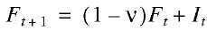
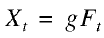
In order to study the influence of fiscal reforms on the national economy, let us use a simple business growth model, which comprises four relations:

                                                                           (1)

                                                                                                    (2)

                                   (3)

                                                                                                     (4)

where F is fixed assets; X is the volume of revenue (production output); I is investment in fixed capital (capital investment); π is net profit; ν is the rate of capital retirement; g is capital productivity ratio; m is the proportion of net profit reinvested in fixed assets; r is the share of net profit in revenue; t is the time (year) index. The coefficients ν, g, m, and r act as model parameters and are assumed to be time–constant.

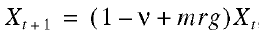
Relations (1)–(4) can easily be reduced to a homogeneous difference equation

                                                                     (5)

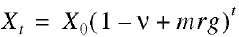
whose solution is given by the following exponential function:

                                                                         (6)

where X₀ is corporate revenue at start time.

If a production growth rate characteristic, λ=X_t/X_t–1–1, is introduced, then the following relation follows from formula (6), which is fundamental for our further analysis:

                                                                                         (7)

Formula (7) relates the rate of economic growth to key reproduction characteristics of the company.

Let us consider an obvious balance:

                                                                                    (8)

where Z is total fiscal costs, i.e., the costs related to fiscal payments; U is other corporate costs (with the exception of total fiscal costs.)

If we pass to the relative values of ɀ=Z/X, и=U/X, and r=π/X, relation (8) can be written as

                                                                                                 (9)

Formula (9) gives the dependence of the rate of return on fiscal and other costs. Further on, the coefficients и. ɀ, and r can be treated as parameters. Combining relations (7) and (9), we obtain the basic equation:

                                              (10)

Therefore, the rate of economic growth depends on the rate of capital retirement (ν) and the productivity (g) of fixed assets, the average propensity to invest (m), the level of specific production (u), and fiscal (ɀ) costs. [1]

The gist of equation (10) is the formalization of the following regularity: any increase of total fiscal costs is actually a decrease in the company’s financial assets intended for maintaining the reproduction process, and therefore, it reduces the rate of economic growth. Proceeding from this analytical construction, we can perform a more proactive analysis of the fiscal reforms.

Note that a similar model was proposed in [1]; in this paper, however, it has a more general form, which makes it universal. Thus, it can be used to analyze the functioning of both material production industries, where fixed assets play a key role, and nonproductive industries. To this end, some of the model variables and parameters are assigned a somewhat different meaning. For example, for enterprises in non–capital–intensive industries, instead of fixed capital, we should use total active financial capital (“working” assets); capital productivity ratio is transformed into the ratio of the corporate revenues to the total financial capital, and the capital retirement parameter turns into the financial assets dissipation factor (capital dispersion and “evaporation” can result from structural inflation and other factors).

Total fiscal costs: economic meaning, structure, and calculation

Equation (10) contains the cost parameter ɀ. Let us explain its content and relation to the fiscal reforms being conducted by the government regulatory agencies.

As already noted, parameter ɀ refers to the costs incurred while effecting fiscal payments. They may be subdivided into two large parts, i.e., fiscal payments (amounts of money paid by the firm to all levels of budgets and to extrabudgetary funds) and the tax administration costs (the costs of tax accounting and compliance with tax payment requirements.) The first component is traditional and is normally used in economic analysis, the second one is rarely recognized and, to the best of our knowledge, its content has been first properly explained in [2]. The consideration of the amount of total fiscal costs [2], including two different components is crucial for our further analysis. In this connection, let us discuss the cost aggregate related to tax administration in more detail.

First, these costs are incurred both by individual taxpayers and the state as a whole. For the state, tax administration includes the upkeep of the respective government agencies, i.e. executive bodies (the agencies responsible for tax collection), legislative bodies (the agencies responsible for rule–making in the fiscal sphere), and judicial authorities (the agencies responsible for settlement of tax disputes between state and taxpayer.) For a taxpayer, this kind of cost includes the costs of tax accounting and bookkeeping [3], tax planning and tax optimization, and various consultations and audits.

Second, the costs of tax administration are incurred by both physical and juridical persons. The main burden of these costs, however, falls primarily on juridical persons.

Third, generally speaking, the tax administration costs of physical and juridical persons include also some “shadow” aggregates. For example, the time spent by individuals on filing their tax returns, on the preparation of required documents and income statement, and the time wasted in the line to the tax inspector’s office are not expressed directly in monetary terms, although this can readily be done, if necessary. Similarly, bribes given by juridical persons to tax inspectors and “protection” racket payments are not included in the company’s accounting costs, although they have a perfectly tangible monetary content. These “shadow” costs must be taken into account in considering the consequences of tax reform.

The introduction of the notion of tax administration costs is not by itself sufficient for understanding how the “shaking” of the fiscal system affects economic growth. To make an in–depth analysis, we need the approach developed in the theory of institutional and technological traps [3–5], i.e., tax administration costs are subdivided into current (fixed) costs and capital (one-time) costs. Current costs correspond to the effective fiscal system capital costs incurred when fiscal reforms are implemented. These concepts are fairly similar to transaction and transformation costs in the theory of institutional traps.

Here, fiscal reforms refer to the transition from one fiscal system to another. In other words, an expanded interpretation of fiscal reforms is applied to allow for any qualitative or quantitative changes in the current system. Even if those changes are not significant, we can refer to them as fiscal reforms since their introduction implies that the system has undergone some transformation. This interpretation automatically leads to the quantitative characteristics of fiscal reforms, i.e., the recognition of the scale and extent of changes in the tax system, which in turn determine the rate of economic growth.

Such an interpretation clears out the difference between current (fixed plus variable) and capital (onetime, transformation) costs of tax administration. Unlike current costs, capital costs include supplementary costs resulting from changes in current regulations, e.g., the costs of new accounting documentation, new accounting software, the adjustment and tuning of available accounting software (programmers’ fees), consultations about new schemes of taxation, the cost of mandatory audits, which previously were unnecessary, the retraining of bookkeeping and accounting staff and their salary increase, etc. When the transition to a new tax accounting system has been completed, capital costs either vanish or become insignificant for the company (k ≈ 0).

To summarize, we can introduce the following expansion for the total fiscal costs Z:

Z_t = C_t + K_t+T_t                                                                                                                                                                           (11)

where С, К are current tax administration costs and one–time tax administration costs; T is the amount of fiscal payments proper (the money paid by the firm to all levels of budgets and to extrabudgetary funds.)

Passing to the relative values с = С/Х, k = K/X, and q = T/X, calculation (11) takes the form

ɀ = с + k + q                                                                                                                                                                              (12)

Then, in view of formula (12), equation (10) will become a little more precise:

           (13)

We now obtain the following simple relation reflecting the effect produced on the rate of economic growth by the fiscal reforms, which modify the parameters of the total fiscal costs and do not affect other reproduction characteristics:

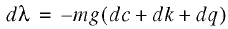                                        (14)

Obviously, formula (14) somewhat simplifies the real mechanism of the effect produced by fiscal reforms. In actual practice, change in the total fiscal costs affects at least one more parameter of the average propensity to invest m. Sometimes, an increase in the total fiscal costs results in the extinction of investment activity (dm/dɀ < 0), and sometimes it leads to the strengthened producer resistance to negative trends (dm/dɀ > 0). Therefore, the complex multicollinearity of the parameters m and ɀ, strictly speaking, makes it necessary to refine equation (14):

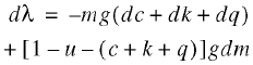                                                     (15)

In the general case, however, it is not possible to predict changes in the relative investment activity, and further on, this effect will not be taken into consideration.

All the calculations made for a single enterprise are applicable to the economy as a whole, but only with an allowance for a certain asymmetry in revenues generated and cost outlay. Thus, the aggregate state revenue is represented by fiscal payments and its net revenue, i.e., the revenue less fiscal payment costs, is the difference between the sum of those payments and the costs of tax administration. At the same time, the latter costs include current and one-time costs. This mechanism could readily be formalized and is largely similar to the corporate model; yet, it will not be considered in this paper.

Classification of fiscal reforms; fiscal quasi– and pseudo–traps

The foregoing concepts and formulas make it possible to take a new view of the fiscal reforms being implemented in Russia. First of all, they should be considered on three adjoining time intervals, including the prereform period (t – 1); the period of the reform implementation (t); and the postreform period (t + 1). This time scale implies a fairly simple and orderly classification of reforms themselves, depending on the development of the total fiscal costs over different time intervals.

The classification criterion is the fiscal reform efficiency for the economy, i.e., its effect on economic growth. In this connection, three obvious types of reform can be singled out.

Globally effective reform. It is characterized by the decrease of total fiscal costs from their initial value both during and after the reform: 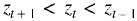. Consequently, such a reform has a positive effect both in the short term (over the time of the reform implementation) and in the longer term (during the postreform period). This reform can be considered effective both from the viewpoint of strategic planning and for the tactics of the state regulatory measures. This process is represented graphically in Fig. la.

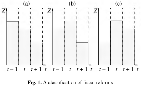
Locally effective reform. It is characterized by the increase of total fiscal costs at the time of reform and their decrease from the initial value after the reform: . Such a reform has a negative short–term effect, but a positive longer term effect. It is therefore effective strategically but ineffective from the viewpoint of the methods for attaining the purpose in view (Fig. lb).

Ineffective reform. It is characterized by the increase of total fiscal costs both at the time of reform and after it: . Consequently, such a reform affects the economy adversely both in the short and long term (Fig. lc).

These definitions are based on the behavior of total fiscal costs. However, in accordance with formulas (11) and (12), this is not a homogeneous value, which enables us to supplement the suggested classification. All the three kinds of fiscal reform can be subdivided into liberal and restrictive. Liberal fiscal reforms are characterized by a decrease in the tax burden (amounts of fiscal payments charged) (dq < 0), and the restrictive reforms are characterized by its increase (dq > 0). In other words, during a liberal fiscal reform, the tax burden decreased from the initial period , and a restrictive fiscal reform leads to a rise in the tax burden .

Therefore, fiscal reforms can differ in their effect on the producer (globally effective, locally effective, and ineffective) and in the implementation method (liberal and restrictive). At the same time, the inefficient restrictive mode is in turn subdivided into two submodes, when the tax burden increase is accompanied by the rise (dc > 0) or fall (dc < 0) in the current costs of tax administration. The latter reform option may be singled out as a separate class, which we will call a fiscal pseudo–trap. What is a salient characteristic of this economic mode?

The fact is, this is the most controversial type of reform. On the one hand, it leads to an increase in the total fiscal costs for the producer and in this regard it is ineffective, but on the other hand, it enables the enterprise to reduce its current tax administration costs, which makes it effective in this respect. What matters is that when, in the course of reform, there is a switch from one method to another (i.e., from the restrictive method to the liberal one), the reform itself can be turned from ineffective into effective. In this regard, one may say that there are certain reserves in implementing this kind of fiscal reform. Although on the face of it this mode of economic development looks like a certain fiscal trap penalizing the producer, actually, it is not so because there are reserves for making the situation better; that is why we classify it as a fiscal pseudo–trap.

Along with the above–mentioned modes of fiscal reform, we can single out one more mode, which is related to, but also distinct from, them. The reference is to a prolonged locally effective fiscal reform. The peculiarity of a locally effective reform is the increase in the total fiscal costs at the expense of one–time costs in the transition period of reform. If the transition period is relatively short, the situation “improves”, and if it is prolonged, this also prolongs the period over which total fiscal costs will exceed their initial level. At first sight, this phenomenon may look like a fiscal trap for the economic system, but actually, this trap is of an artificial nature and should be more properly termed a fiscal quasi–trap. Essentially, this mode implies that this ineffective state terminates as soon as the reform, constantly generating one–time tax administration costs, has been completed. Therefore, when a fiscal reform, even if essentially effective, turns into a permanent process, this leads to the formation of a certain fiscal quasi–trap. In this case, a connection between the government reforms and such a phenomenon as an institutional trap can be observed: continuous reforms may grow into quasi–traps, which are not easily distinguished from ordinary institutional traps.

Explanation of fiscal paradoxes in terms of fiscal traps

The above analytical scheme and the concepts introduced allow us to expound on the processes that have taken place in Russia over the last decade. The central phenomenon calling for explanation is the inefficiency of fiscal reforms being implemented in Russia. For instance, Russian authorities, aware of the necessity of lightening the domestic producer’s burden, were constantly trying to improve the situation by endless tax rebates and refining the taxation procedure; every single year during the previous decade and a half, serious changes were introduced in the tax legislation. Thus, according to Bureau of Economic Analysis (BEA) data for 1991–1999, profits tax laws were changed 15 times, there were 16 different wordings of the income tax law, and the same number of wordings of the VAT law [6, p. 144]. At the same time, those “favorable” changes either aggravated the producers’ position or had no stimulating effect at all. How can this paradox be explained and is there any reasonable interpretation of this situation?

One of the possible answers is mistakes made in amending tax laws. Up to the present, many specialists believe that all the liberal fiscal concessions made by the authorities were offset by restrictive measures. We do not believe this is the case. It would be more reasonable to assume that the development of market–oriented accounting practices in this country, with its complex tax legislation, was accompanied by the slow but steady escalation of tax administration costs (i.e., the inequality dc>0 obtained). The iterative pattern of reviews of tax accounting regulations led to increases in the current (fixed) costs of tax administration. Simultaneously–and this is of greatest importance–continu­ous changes in accounting standards generated considerable one–time costs of adjustment to the new system (dk>0).The fiscal reforms, dragged out for 15 years, added an ever–present transformation element to tax administration costs (k>0).

Therefore, fiscal reforms brought about a significant increase in the corporate tax administration costs. The reforms never ended, thus preventing producers from “removing” part of their administrative costs and thereby improving their position. By some estimates, extra costs incurred by companies in connection with tax compliance and related formalities may reach 15–30% of the tax amount [7, p. 46]. Against this background, the lightening of the tax burden (dq<0), in the first place, was not always been consistent enough (with periods when the inequality dq<0 obtained alternating with periods when dq>0), and in the second place, it could not fully compensate for increases tax administration costs (dq+dc+dk>0). The endless reproduction of this situation led to the formation of a fiscal quasi–trap, which was characteristic of the entire transition period. It can reasonably be assumed that this process is still going on.

In summary, we can state that the prolonged reform of the Russian taxation system has gradually assumed the form of a fiscal quasi–trap and thereby hinders the activization of the domestic producer at the initial stage of economic reforms. The evident conclusion is that the national fiscal system will become efficient only when its reforming has been finalized and all the quantitative and qualitative parameters are stabilized, which will mean that the formed fiscal quasi–trap has been removed.

Potential of fiscal quasi–traps: quantitative pattern

In order to measure the pressure of fiscal reforms on producers, some calculations, however tentative, should be made. This can be done using a simplified variant of formula (14): Δλ = –mgΔk.

This accounting scheme is based on the assumption that the tax burden and current costs of tax administration stay unchanged throughout the fiscal reform period. For simplicity, it will also be assumed that the entire net profit generated by a company is reinvested in production expansion (m = 1), and capital productivity is 0.3 (it is a typical value if the output is calculated relatively as generated value added).

At present, there are no reliable statistical data about tax administration costs and, consequently, about parameters с and k. We will, therefore, proceed from the above figures, according to which the cost parameter (c + k)/q varies within the 15–30% range and the tax burden q is at the rate of 30% of value added. Assuming the averaged estimate of (c + k)/q to equal 20% and assuming that fiscal reforms increase it up to 30%, it can readily be calculated that such a “blow” dealt by fiscal authorities would reduce the economic growth rate by 1 percentage point. If we assume that the initial value of (c + k)/q was 10% and the fiscal reforms raised it to 30%, the “shrunk” economic growth rate would be 2 percentage points, which corresponds to the “natural” or “normal” rate of economic growth.

How can we assess these estimates of the pressure exerted by the fiscal quasi–trap?

At first glance, these figures are not very impressive. Indeed, for the Russian economy at the time of transformation recession, such effects could not be considered to be of critical importance. Clearly, such effects aggravated the crisis but their contribution was by no means crucial. The situation changes significantly if we consider more normal and stationary economic conditions. Thus, at the time when the economy is passing from recession to growth and when this growth amounts to fractions of a percent, its decline by 1–2 percentage points can delay the economy’s surmounting the recession. If economic growth is modest, the pressure of fiscal reforms can be significant enough to “knock production down” it and would either lead to its stagnation or plunge it into a new recession. Moreover, it should be taken into account that the fiscal quasi–trap formed in Russia generates a permanent (annual) “overhang” above the economic growth rate of 1–2 percentage points, which in five or six years, could amount to a tan–gible figure of 10% GDP the country would lose because of continuous fiscal reforms. Therefore, we should not downplay the impact of the fiscal quasi–trap.

More correct applied calculations on a larger scale cannot be made at present since there are no official or reliable statistics of tax administration costs. We believe it would be advisable to add this index to practical statistical accounting because it can provide important information not only about companies and enterprises, but also about the efficiency of the fiscal reforms implemented in the country.

Acknowledgments

The author thanks Yu.V. Kuznetsov for a useful discussion of this paper.

References

1. E. V. Balatskii, “Reproduction Cycle and Tax Burden,” Ekon. Mat. Met., No. 1 (2000).

2. Yu. V. Kuznetsov, “What We Do Not Know about Taxes,” Otechest. Zap., Nos. 4–5 (2002).

3. V. M. Polterovich, “Institutional Traps and Economic Reforms,” Ekon. Mat. Met., No. 2 (1999).

4. E. V. Balatskii, “Functional Properties of Institutional Traps,” Ekon. Mat. Met., No. 3 (2002).

5. E. V. Balatskii, “Economic Growth and Technological Traps,” Obshchestvo Ekon., No. 11 (2003).

6. S. B. Avdasheva, S. A. Afontsev, V. G. Voronina, et al., Review of Russia’s Economic Policy in 2003. Economic Analysis Bureau (TEIS, Moscow, 2004) [in Russian].

7. S. B. Avdasheva, E. I. Andreeva, V. D. Andrianov, et al., Review of Russia’s Economic Policy in 2002. Economic Analysis Bureau (TEIS, Moscow, 2003) [in Russian].