
There is a growing interest in the study of the role of fiscal factors in government regulation. Close attention is being paid to the properties of the Laffer curve. One drawback common to this body of work is perhaps excessive theorizing, which in a vast majority of cases denies the possibility of correct applied computations. The prevailing negative trend complicates macroeconomic analyses and forecasts of the development of the national economy.
Meanwhile, the practice of macroeconomic decisions is pressing for a toolkit to permit the assessment, with a sufficient degree of confidence, of the fiscal policy of a state in terms of its impact on the level of business in the country. What is needed in fact is a toolkit that helps determine the shape of production and fiscal curves and estimate their flex points, i.e., Laffer points of the first and second kind respectively.
Without attempting an excursion into the history of taxation, we merely wish to note an interesting fact. The idea of the optimal level of tax load, the Laffer curve, originated in the United States. Afterwards, however, this concept was used for the most part as an element of more general econometric models. In particular, Buchanan’s, Monissen’s, and some others’ studies [1–4] follow this line of thought. At present. Western economic theorists are rather critical of the Laffer curve concept. By contrast, there are numerous papers by Russian economists dealing with the geometric properties of this curve. Suffice it to say that the very idea of the Laffer point originated with Russian researchers [5]. Subsequently, this notion was repeatedly refined [6–9], notably by the introduction of Laffer points of the first and second kind [8]. A parallel effort was to develop various methods and algorithms of their identification [8, 10]. This paper is the next step toward determining the instrument base of the macroeconomic framework of the Laffer curve. We must make an important reservation: by focusing on computation problems, we deliberately abstract from many–sometimes, even very important–theoretical fine points of this concept for fear of drowning the gist of the matter in particulars.
Production–institutional functions: their essence, features, and philosophy of application to the study of fiscal climate
Production–institutional functions are the core of the proposed model analysis of fiscal climate. Let us examine features of this model apparatus.
To begin with, production–institutional functions are an extension of the conventional production function (PF) apparatus to the macrolevel. The only difference is that conventional PFs use output for the endogenous indicator (as a rule, GDP volume) and for macrofactors, labor (employment volume) and capital (fixed assets), whereas in production–institutional functions the set of macrofactors is augmented by variables characterizing the production environment. We shall consider a single institutional variable, average tax load, i.e., the share of taxes levied by the state in the GDP. Given that our model, in addition to the purely technological (resource) aspect of economic growth (labor and capital volumes and efficiency), also recognizes institutional climate (tax burden), the conventional PF is accordingly transformed into a production–institutional function.
Investigating the production–institutional function appears to be reasonable in view of the fact that the relationship between output and macrofactors is largely determined by the economy’s prevailing institutional climate. It seems logical to assume that the technological conditions (labor and capital volumes) being equal, different tax loads produce different GDP volumes. Taxes, by contributing to the formation of the economic agents’ system of incentives, have a direct bearing upon the level of the business, hence production, activity of a system.
The idea of development of production–institutional functions is not new. In 1994, Welfens and Jasinski proposed the use of an “extended” Cobb–Douglus function as a purely theoretical construct, which involved an exponential factor depending on several institutional parameters [11]. Besides, the present–day econometric practice indicates that factors of production are often represented not only by resource variables but also by government regulation parameters such as interest rates, tax burden, etc. [12].
However, the examination of a three–factor (labor, capital, and tax load) production-institutional function is, generally, insufficient fora nontrivial analysis of fiscal climate and the assessment of its role in sustaining economic growth. We must assume that the relation between output and tax load is nonlinear. Besides, it makes sense to consider not conventional PFs with a constant elasticity of substitution of macrofactors, but PFs with a variable elasticity, which itself depends on tax load. In this case, the institutional factor is not merely added to the econometric model but is directly interwoven with the net of technological links. This model design allows the most comprehensive analysis of the role of fiscal climate.
Fiscal analysis methodology using production–institutional functions
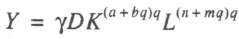
Let us elaborate on the foregoing with reference to specific functional relations. To do so, we use a production–institutional function of the form
 (1)
(1)
where Y is output (GDP of the country); К is capital (fixed assets); L is labor (economy workforce); q is tax load (relative tax burden computed as the share of tax proceeds T in GDP, q = T/Y); D is a trend operator (a function depending on time t); γ, α, b, n, and m are statistically estimated parameters based on retrospective time series. The variables Y, K, L, and q are taken for the respective years t.
A characteristic of function (1) is that a country’s macroproduct depends on labor, capital, and tax burden, with the influence of labor and capital on economic growth itself depending on fiscal climate. Furthermore, labor and capital elasticities are quadratic functions of the tax load, which automatically predetermines the nontriviality of the whole analysis.
Note that functions with variable elasticity of factor substitution are rather uncommon in econometric practice. Yet, as shown by empiric computations, this form of the production–institutional function is not only the most acceptable but also quite general.
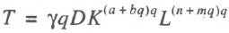
Function (1) sets the production curve, i.e., the relation between output and tax load. Then, the fiscal curve, i.e., the relation between the mass of collected taxes and relative tax load, is described by the functions
 (2)
(2)
The pivotal idea of fiscal analysis based on production–institutional functions (1) and (2) is to determine the relative position of the Laffer points of the first and second kind and the actual size of the tax load. When the data of three fiscal indicators are examined, one can draw a fairly complete picture of the fiscal climate and its role in shaping economic growth dynamics.
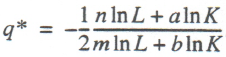
According to a classification proposed in [8], a fiscal Laffer point of the first kind, q*, is the peak (i.e., maximum point) of production curve (1), when dY/dq = 0. After simple transformations, we can write an explicit expression for the Laffer point of the first kind of function (1):
 (3)
(3)
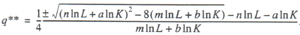
Similarly, we determine the fiscal Laffer point of the second kind, q**, which we interpret as the peak (i.e., maximum point) of fiscal curve (2), in case that dT/dq = 0. Simple computations lead to the following formula for the Laffer point of the second kind of function (2):
 (4)
(4)
Formula (4) calls for some explaining. From two critical points, determined according to (4), we select the maximum point. However, one cannot say in advance which of the two critical points will be the maximum one, and this explains why formula (4) includes two potential Laffer points of the second kind.
The right–hand sides of (3) and (4) depend not only on the model parameters but also on instrumental variables, which in turn depend on time; therefore, Laffer points of the first and second kind themselves are not constant over the total study interval. On the contrary, they are “floating” in time, which is a great advantage of this analysis. Indeed, it is more in order to suppose that the sensitivity of the economic system to the tax burden is a dynamic value varying from year to year.
Another important positive characteristic of production–institutional functions (1) and (2) is that the Laffer points of the first and second kind, (3) and (4), are invariant relative to the trend operator, D. The fact is that when relationship (1) is adapted to specific statistical data, the particular shape of the function of the trend component, D, may change. Thanks to the manipulation of the functional relationship D = D(t) we can fit approximating function (1) to the specificity of concrete time series with sufficient accuracy. From a substantial point of view, the relationship D = D(t) describes neutral scientific and technological progress.
However, despite the fact that the functions of the trend D = D(t) vary in different applied calculations, Laffer points of the first and second kind prove to be independent of its parameters. In other words, a method for determining fiscal indicators by formulas (3) and (4) helps eliminate the distorting influence of STP and the time factor in fiscal analysis.
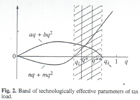
Econometric model (1) involves another important angle of the macroeconomic analysis at hand, which merits special consideration. The point is that this form of relation is impossible without a close linkage of technological and fiscal factors of economic growth. It manifests itself, in particular, in that the character of influence of labor and capital on output (the sign of the derivatives ∂Y/∂K and ∂Y/∂L) is nonlinearly dependent on tax burden. This fact assumes the introduction in the analysis of two more fiscal indicators as crossing points, qK and qL, corresponding to the stationary conditions ∂Y/∂K = 0 and ∂Y/∂L = 0:
qK = –b/α (5)
qL = –m/n (6)
If the parabola αq + bq2 is upward convex, then, with a tax load less than level (5), the marginal productivity of capital is positive and any increase of fixed assets leads to production growth. If the tax load proves to be above point (5), the marginal productivity of capital turns negative and an extensive increase of this factor merely induces a production recession. If the parabola αq + bq2 is downward convex, the situation is diametrically opposite. Similar reasoning is applied to the crossing–point, (6). Therefore, technological and fiscal analyses turn out to be coincident, with technological characteristics such as marginal productivity of labor and capital being directly dependent on tax load.
In examining the interrelations of fiscal and technological factors, the index of elasticity of substitution of labor for capital, E = (L/K)(dK/dL), assumes independent importance:
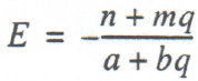 (7)
(7)
Thus, the whole methodology of the proposed analysis consists in examining six indicators: the actual tax burden, q, and indicators (3) to (7). The set of these characteristics, inclusive of the geometric properties of curves (1) and (2), allows quite accurate diagnoses of fiscal climate and its role in the development of a particular economic growth path.
Given the role in our analysis of the measure of tax load, q = T/Y we shall make a few observations on special features of its calculation. The fact is that only the actual tax load, i.e., the share of fiscal withdrawals from the GDP that in the final count was contributed to the public budget, is recorded in this form. The nominal tax load, i.e., the share of value added produced, which should have been withdrawn to the budget under active legislation, may be significantly higher [13]. The actual tax load, q, is what is vitally important to the producer, which is recognized in our scheme. Indeed, when examining production dynamics in retrospect, it is in order to assume that it was determined by how much the producer paid in taxes and not how much he was supposed to pay. In this context, the size of the nominal tax burden is largely a virtual quantity, which, given today’s production decisions, is “suppressed” by the present–day actual tax burden.
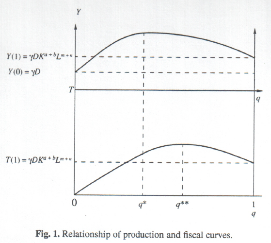
From the point of view of theoretical “purity” functions (1) and (2) can be considered rather good. For instance, in the absence of either of the two resource factors (L = 0 or К = 0), production according to (1) is impossible (Y = 0), which meets the canonical requirements imposed upon production functions (tax proceeds, correspondingly, also equal zero). The behavior of functions (1) and (2) at the ends of the fiscal parameter q is much more interesting. In the absence of taxes (q = 0) output equals Y = γD and fiscal returns are lacking: T = 0. Therefore, the fiscal curve at its leftmost point behaves according to natural economic logic and thus satisfies the postulates of the classical supply theory. The production curve at this point is not vanishing, as proposed by conventional theory; however, as shown in [7], this demand is too steep and we can consider it quite normal that output at this point takes on some conventional small value. At the rightmost point q, when all the earnings are withdrawn as taxes (q = 1), the amounts of output and fiscal charges logically coincide (Y = T), with Y = γDKα+bLn+m. Although this value is not vanishing, as assumed by the orthodox supply–side economics, at respective values of parameters it may be arbitrary close to zero. Therefore, from the point of view of the theoretical standard, the behavior of the production and fiscal curves on the right–hand border can be considered perfectly satisfactory; a schematic of the production and fiscal curves is shown in Fig. 1.
Having chosen function (1) as our main analytical tool, we will make a few more observations. First and foremost, theoretical constructs in a number of cases assume that fiscal policy is a long–term, rather than tactical, instrument of macroeconomic regulation. It means that a change in the tax load will redound upon the level of business not so much in the current year as in the years to come. We feel that this proposition is debatable. It would seem to be right to presume that any–especially a sharp–change in tax burden will affect the level of business already in the current year. Perhaps it makes sense here to speak about the distribution of the fiscal effect year by year. However, hereafter we will proceed from the assumption that the establishment in practice of a satisfactory lag–free econometric relationship, (1), is sufficient grounds for rejecting the use of similar time–lag models.
The variables K, L, and q are assumed to be independent, as function (1) itself describes job formation, and in view of the continuing unemployment it is job offer, not job demand, that is the limiting factor of economic growth. In other words, the possible influence of q on labor supply is not decisive, because at the macrolevel, labor supply is less than labor demand anyway.
Now, let us discuss the terminology itself. The Laffer points of the first and second kind that have been introduced reflect inflection effects in the respective curves and are to some extent technical. They were introduced in view of the postulate of such effects that is pivotal in Laffer’s conception. Yet inflection mechanisms may vary. This fact is not, of course, recognized in model (1) and in the terms introduced.
Results of the econometric rating of the three–factor production–institutional function
To validate function (1) we used statistical data from four countries: Russia, Sweden, the UK, and the USA. The choice of these countries was motivated by the desire to obtain the most representative sample, which includes all the principal types of economic systems. For instance, the British economy is quite “old” with a rather conservative government regulation system and a moderate fiscal load. What makes Sweden interesting to us is its famous model of “Swedish socialism,” which depends on a very high tax burden. The United States, by contrast, is representative of a group of countries with liberal tax regulations and a very flexible system of macroeconomic regulation. Lastly, Russia belongs to developing countries and transition economies, characterized by instability both of their economic processes and regulation systems. The examination of such different classes of national economies is of itself a very good test for the generality of the proposed econometric relationship (1).
As already mentioned, the chief “national” singularity of function (1) is the method of accounting for scientific and technological progress. Yet, studies have shown that there is a pattern here, too. In particular, for each of the countries concerned, the trend function can be presented in the following general form:
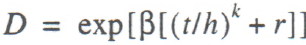 (8)
(8)
where t is time (year); h, к, and r are parameters antecedently defined for each country with a view to improving the quality of process approximation; β is an econometric parameter defined statistically on the basis of retrospective time series.
In point of fact, the form of accounting for STP (8) is a generalization of Tinbergen’s neutral STP; at h = к = 1 and r = 0, expression (8) takes on the canonical form of Tinbergen’s trend multiplier: D = expβt. Table 1 lists the values of the antecedent parameters of the STP function for different countries.
Table 1. Parameters of STP trend function (8) for different countries
|
Country |
STP parameters |
||
|
h |
к |
r |
|
|
Russia |
100.0 |
0.2 |
0.00 |
|
Sweden |
3000.0 |
0.0 |
0.03 |
|
Britain |
1000.0 |
0.0 |
0.00 |
|
United States |
100.0 |
1.3 |
0.00 |
By taking the logarithm, model (1), with allowance made for (8), can be reduced to a linear function with regard to its parameters. Table 2 lists the results of an econometric rating of function (1) for the countries in question. In some cases, the units of measurement of labor and capital are chosen so as to bring the two factors to the same magnitude.
Table 2. Parameters of econometric model (1)
|
Coefficient |
α |
β |
n |
m |
|
b |
|
Russia. 1989–2000 |
|
|
|
|
|
|
|
Value |
5.19 |
–0.74 |
8.45 |
–11.38 |
–3.77 |
5.06 |
|
t–Statistic |
2.94 |
–1.47 |
1.19 |
–0.52 |
–0.79 |
0.38 |
|
Statistical parameters |
|
R2 = 0.979; DW = 2.35; N= 12 |
|
|||
|
Sweden. 1980–1994 |
|
|
|
|
|
|
|
Value |
0.11 |
37.24 |
–3.05 |
4.98 |
3.87 |
–6.69 |
|
t–Statistic |
0.29 |
36.47 |
–5.36 |
4.97 |
5.77 |
–5.08 |
|
Statistical parameters |
|
R2 = 0.998; DW= 3.21; N= 15 |
|
|||
|
England, 1983–1999 |
|
|
|
|
|
|
|
Value |
–0.21 |
15.03 |
–4.61 |
8.11 |
1.72 |
–1.88 |
|
t–Statistic |
–0.16 |
13.81 |
–1.12 |
0.73 |
1.14 |
–0.49 |
|
Statistical parameters |
|
R2 = 0.998; DW = 2.14; N = 17 |
|
|||
|
United States, 1986–2000 |
|
|
|
|
|
|
|
Value |
–4.56 |
0.22 |
–33.18 |
127.63 |
14.98 |
–45.87 |
|
t–Statistic |
–0.69 |
0.16 |
–1.87 |
2.08 |
1.93 |
–2.07 |
|
Statistical parameters |
|
R2 = 0.999; DW= 2.01; N= 15 |
|
|||

Note: α = lnγ.
The econometric assessment time spans were chosen based on information available. Two conditions had to be met: the length of a series must not be too great (not to exceed 17 years), otherwise calculation accuracy will suffer, and analysis periods must be as close to current year as possible, since an in–depth study of earlier historical intervals is an independent task. Observing these principles automatically ensures the comparability of place–to–place computations and furnishes an objective basis for searching for developmental features of each national economy.
We encountered no problems in constructing retrospective statistical arrays of Y and L. When estimating К, however, Sweden and Britain posed an information and methodological problem because these countries do not record the value of fixed assets; in Sweden, it was not until 1995 that statistical offices began to monitor this indicator. In view of this, we used the index of capital expenditure for the Swedish and British economies. Given the high interdependence of the measures of fixed–capital stock and capital expenditure, this replacement did not affect applied calculations. [1]
There are different approaches to the calculation of tax load, q. One approach includes the stripping of the total budget revenue of income tax so as to arrive at the tax load upon the producer proper. This approach was applied to Russia, whereas in the case of other countries, income tax was included in the resulting tax load.
Using different schemes of estimation of the actual tax burden is in the nature of a modeling experiment, the underlying reason being the special role of the income tax on natural persons. The point is that in several countries, workers themselves pay the income tax. In the case of the progressive tax, which was in effect in Russia in 1989–2000, and given several sources of income, natural persons themselves pay the rest of the income tax. Besides, in the functional plane, corporate entities’ taxes influence mainly job offer, whereas the taxes of natural persons influence job demand. The foregoing suggests the idea of splitting all taxes into corporate taxes and individuals’ taxes.
By and large, our computations demonstrated that function (1) is well suited for the description of economic growth in all the above countries. Given minimal calibration of trend function (8), model (1) approximates real–life processes with a high degree of accuracy. Sweden is perhaps the only exception, for which the Durbin–Watson coefficient leaves much to be desired, but given the limiting value of the coefficient of determination (R2 = 0.998), this fact does not cause any computation problems (Table 2).
Therefore, model (1) passes all the statistical tests for each of the four countries and can be accepted as workable. The generality of model (1) can thus be considered proven and its underlying approach, which assumes a synthesis of technological and fiscal factors, perfectly legitimate.
Specificity of the transformation setback in Russia: empiric results
Once function (1) has been identified, we can pass over to the main problem, the analysis of the tax factor in the growth path formation.
Let us consider this question with regard to Russia. Table 3 summarizes calculations by formulas (3), (4), and (7). Let us analyze special features of the Russian economy in the period 1989–2000.
Table 3. Fiscal and technological indicators of the Russian economy, %
|
Year |
q* |
q** |
q |
E |
|
1989 |
36.59 |
46.22 |
30.95 |
2.23 |
|
1990 |
36.57 |
46.39 |
35.64 |
2.23 |
|
1991 |
36.55 |
46.67 |
32.19 |
2.23 |
|
1992 |
36.52 |
47.08 |
36.03 |
2.23 |
|
1993 |
36.49 |
47.44 |
29.53 |
2.23 |
|
1994 |
36.45 |
48.03 |
30.33 |
2.23 |
|
1995 |
36.44 |
48.15 |
26.27 |
2.24 |
|
1996 |
36.42 |
48.37 |
30.15 |
2.23 |
|
1997 |
36.38 |
48.94 |
33.39 |
2.23 |
|
1998 |
36.35 |
49.30 |
29.62 |
2.23 |
|
1999 |
36.42 |
48.32 |
31.39 |
2.23 |
|
2000 |
36.44 |
48.09 |
34.63 |
2.23 |
To begin with, what strikes the eye is the superhigh stability of the Laffer point of the first kind: during 12 years, its value ranged from 36.35 to 36.59%. Therefore, fiscal variation throughout these years was negligible, 0.24%, and we can estimate the value of the Laffer point of the first kind in Russia within very small limits–36.5%.
This high stability of q* gives evidence, first and foremost, of the stability of the propensity of Russian producers for marginally permissible fiscal costs. In our case, this quantity is far above one–third of the value added and close to the US “empiric 35% standard.” This kind of stability of producer psychology is somewhat paradoxical at first sight. Indeed, the transition period, with its inherent randomness of all processes and the uncertainty of the future, should have produced a totally different result, a constantly fluctuating Laffer point of the first kind with a rather big amplitude. We believe that the actual cause of stability in user psychology was the absence of “secular” trends of production technologies; this proposition will be substantiated below.
Second, figures in Table 3 show a rather high stability of the Laffer point of the second kind, which fluctuated over the range of 46.22 to 48.94%. Therefore, the fluctuation band was only 2.72%, which, given the value of the point q** itself, seems to be quite narrow for this kind of fiscal measure. Based on the mean value of q**, about 47%, we can affirm that in the short term, any increase of the producer’s tax burden will have only a good impact on the Russian budget. Besides, the variation of the Laffer point of the second kind of itself clearly tended to grow. It means that the “reliability” of the tax component of the Russian budget was growing slowly but steadily.
Third, the actual tax burden throughout these years was below the Laffer point of the first kind, let alone of the second kind (Table 3). This proposition is very important as it means the following: in none of the years of the transformation period was the tax burden in Russia excessive, nor was the tax burden so high as completely to shut off the feeding for Russian producers and provoke a recession. It could happen if the actual tax load had exceeded q*. In geometric terms, the Russian economy would then have moved to the descending branch of the production curve. Never once did this happen. Therefore, the fiscal climate in the Russian economy in transformation should be conceded, with a degree of caution, to be perfectly normal and the tax load, moderate.
This fact makes it possible to rethink the transformation downturn phenomenon in Russia. For example, it is now traditional to assume that the ten–year decline in production was due to institutional factors, first and foremost, an institutional demolition of the planned economy. Without calling in question the gist of this proposition, we can still contend that an institutional factor such as taxes did not put as much pressure on the domestic economy as popularly believed. Institutional factors might have played a leading role in the appearance and development of an economic crisis, but the fiscal factor was certainly accidental to that process.
Fourth, the Laffer point of the second kind was all the time significantly higher than the Laffer point of the first kind. The “fiscal gap” between them averaged 10–12% (Table 3). What it means in essence is that even if the state “tightened up” taxes so much that q exceeded the Laffer point of the first kind, it could afterwards continue to raise them by about 10% without jeopardizing budget revenues. Simply stated, government agencies may, without much scruple, force up the tax load to 40% of GDP. This would deal a serious blow to the rate of economic growth, but fiscal revenues would rise anyway. This fact once again proves that the Russian state has largely underutilized its fiscal instruments.
If the foregoing reasoning is correct, the question emerges: If the fiscal factor was not decisive in the origin and “sustenance” of the economic crisis, what is its true nature?
The econometric model used is too aggregated and simple to yield a detailed answer. Nevertheless, it does permit a few important statements to be made.
To begin with, we shall take advantage of the additional information borne by the turning–points, qK and qL. Their calculated values for Russia are: qK = 15% and qL = 74%, with the marginal productivity of labor being positive and the marginal productivity of capital being negative. It means that marginal return on capital may only be positive with a tax burden of 75% of GDP. However, in that case, marginal productivity of labor becomes negative, i.e., one problem is replaced by another, no less complex. Besides, such fiscal costs are beyond the limits of actually permissible values.
Therefore, the Russian economy is operating with one of its macrofactors being absolutely inefficient and its tax instruments unable to normalize the resulting factor imbalance.
It follows that the bottleneck of the Russian economy is its fixed assets, whose extensive rise fostered a production downturn. The analysis period saw a surprisingly inexpedient dynamics of macroresources: employment, contributing to GDP growth, was steadily dwindling, and fixed capital stock, impeding output growth, was steadily rising. Therefore, the transformation decline in Russia had a resource and technological origin.
Overaccumulation of inefficient fixed capital stock is known to be behind any crisis, and Russia has traditionally pursued an irrational investment policy. At present, the country faces the task of an accelerated disposal of outdated productive facilities and the parallel substitution of advanced equipment. The role of the fiscal factor in this process appears to be minimal.
We note in addition that for 12 years in the last century, the elasticity E of substitution of labor for capital was, first, positive, which is evidence of a frankly abnormal relationship of key macrofactors, and second, invariable in size (Table 3). The second aspect is particularly interesting as it unambiguously indicates that the nation lacked direction in scientific and technological progress. Since the fixed capital factor was superfluous, it would be legitimate to suppose that, in these conditions, STP should have a labor–intensive direction. Consequently, E should have decreased, approaching a natural negative value. This was not the case. On the contrary, the “dead center,” E = 2.23, was stable to two decimal places throughout these years. Leaping ahead, we can state that nothing like this “calm” in the field of STP has ever been observed in any other country under review.
Thus, the protracted pattern of the Russian transform action crisis was due not so much to the pressure of taxation on the producer as the technological backwardness of available productive facilities and the lack of a mechanism for STP activation. Understandably, given such conditions the best fiscal climate could not reverse the prevailing negative trend. Variant calculations by model (1) at different values of tax load bear out this conclusion. Let us dwell on this aspect of the problem.
Our computer experiments sought answers to the question: Could a more moderate tax load on the producer reverse the transformation decline? If it could, at what value of the tax burden could the “turning effect,” i.e., the changeover from recession to expansion, be achieved?
To answer these questions we kept the values of the labor and capital factors in function (1) and varied the tax burden. To improve the demonstrativeness of our findings we kept the index q in each scenario unchanged throughout the years of analysis. A total of seven scenarios were examined: q = 0; q = 15%; q = 20%; q = 25%; q = 30%; q = 35%; and q = 40%.
Without giving specific quantitative calculations we shall limit ourselves to a qualitative pattern of the process. In none of the examined scenarios can the anticipated economic reversal be discerned; all the GDP paths have roughly the same shape. It means that no reduction of the tax burden, down to a purely hypothetical scenario of its complete abolition (q = 0) could prevent an incipient downturn. Therefore, real problems of economic crisis should least of all be sought in the fiscal sphere. What is more, according to our computations, the higher tax load options (q = 35% and q = 40%) proved to be even preferable to more liberal fiscal regulations. The point here is that the taxes on the ascending arc of the Laffer curve (up to 36% of GDP) had a stimulating effect and their reduction, contrary to expectations, would likely have led to an even deeper recession. As statistical reports accumulate, we can improve the accuracy of our calculations and results. Meanwhile, we can as well accept the proposition (even in a tentative form) that the Russian economic crisis of 1989–2000 was not of a fiscal nature.
Place–to–place differences of fiscal systems: empiric findings
Our analysis raises the following questions: How specific is Russia’s development compared to other countries? and. Have national fiscal systerns anything in common with regard to structure and nature?
To answer these questions, let us look at the British economy. Table 4 lists calculated data, leading one to a few interesting conclusions.
Table 4. Fiscal and technological indicators of the British economy, %
|
Year |
q* |
q** |
q |
E |
|
1983 |
35.51 |
38.05 |
38.20 |
1.51 |
|
1984 |
35.56 |
38.11 |
38.80 |
1.48 |
|
1985 |
35.59 |
38.14 |
38.10 |
1.52 |
|
1986 |
35.61 |
38.15 |
37.70 |
1.54 |
|
1987 |
35.66 |
38.20 |
37.60 |
1.55 |
|
1988 |
35.75 |
38.28 |
39.90 |
1.58 |
|
1989 |
35.81 |
38.34 |
36.30 |
1.61 |
|
1990 |
35.81 |
38.35 |
36.40 |
1.61 |
|
1991 |
35.75 |
38.30 |
35.20 |
1.66 |
|
1992 |
35.72 |
38.26 |
33.90 |
1.72 |
|
1993 |
35.71 |
38.24 |
33.30 |
1.75 |
|
1994 |
35.74 |
38.27 |
34.30 |
1.71 |
|
1995 |
35.76 |
38.29 |
35.30 |
1.66 |
|
1996 |
35.79 |
38.32 |
35.20 |
1.66 |
|
1997 |
35.84 |
38.37 |
36.50 |
1.60 |
|
1998 |
35.90 |
38.42 |
37.00 |
1.58 |
|
1999 |
35.91 |
38.44 |
36.90 |
1.58 |
First, the British economy exhibits very stable Laffer points of the first and second kind. For instance, the first of them never fell outside the range of the interval of 35.51–35.91%, while the second stayed within the bounds of 38.05–38.44%. Correspondingly, the variation of the Laffer point of the first kind was only 0.40% and that of the second kind, 0.39%. This stability suggests a peculiar immutability of the fiscal attitudes of British society. Against the background of such “internal” fiscal characteristics as Laffer points of the first and second kind, the actual tax burden had a more unstable dynamics over the range of 33.30 to 38.80% with a respective 5.5% variation. In other words, a noticeable adjustment of the real tax climate in Britain occurred against the background of virtually invariable threshold fiscal standards of a traditionally conservative economy.
Second, it is a very curious fact that the “fiscal gap” between the Laffer points of the first and second kind was about 2.5%, which seems a truly paltry quantity, especially in comparison with the Russian one, which was one order of magnitude higher. On average, the Laffer point of the first kind was 35.7% and of the second kind, 38.2%. Thus, the first point almost coincides with the “35% empiric standard,” while the second point is very close to it. The foregoing leads one to maintain that the reaction of a national budget is little different from that of a user. In other words, as soon as the tax burden rises to a point where it exerts a destimulating effect on the producer, almost at once the fiscal revenues of the state begin to fall, i.e., the British fiscal authorities, unlike Russian ones, have practically no degree of freedom in manipulating tax rates. They must concentrate on the producer because his reaction will be automatically reproduced by the national budget.
Third, the effectiveness of the British government’s fiscal policy varied at the different intervals of the analysis period. For example, the period 1983–1984 was characterized by a very high tax burden, when actual tax load exceeded the Laffer point of the second kind (Table 4). In those years, the state in fact defeated its own purpose, and hence, the fiscal policy at that stage can be seen as inefficient or erroneous. The period from 1991 to 1996, by contrast, was marked by a frank liberalization of the tax policy, when the actual tax burden was below the Laffer point of the first kind (Table 4). This “fiscal thaw” exerted a positive influence upon economic dynamics. Two other intervals, 1985–1990 and 1997–1999, were characterized by a moderately depressive fiscal policy, when the actual rate of tax burden ranged between the Laffer points of the first and second kind (Table 4). In those years, taxes roundly curbed production, yet not so much as to “kill” the nation’s budget. This policy should be considered onesided because in this case the interests of the budget are upheld at the producer’s expense. By and large, the 17 years reviewed were a period of an active search by the British government for the most acceptable fiscal treatment. There was a distinct tendency toward “fiscal squeeze” and the curbing of economic growth.
There are objective reasons behind the inconsistency of the fiscal policy pursued by the British authorities. The British economy has in fact operated in conditions of a technological imbalance of macrofactors, which was in a way a mirror reflection of the Russian situation. To wit, if the Russian economy functioned under a negative marginal productivity of capital (∂Y/∂K < 0) and positive marginal productivity of labor (∂Y/∂L > 0), the situation in Britain was the exact reverse: a positive marginal productivity of capital (∂Y/∂K > 0) and a negative marginal productivity of labor (∂Y/∂L < 0). As qK = 91 % and qL=57%, there was in Britain, as in Russia, no sensible taxation climate to help eliminate the resulting imbalance. The problem of inefficiency of direct labor redounded upon the elasticity of substitution of labor for capital, which remained positive throughout. In this respect, Britain’s only advantage over Russia was a smaller and more flexible E (Table 4).
The mirror effect of the technological structure of the Russian and British economies points to profound differences between the two systems of management. For example, the main driving force of the British economy is a fairly efficient capital, while labor is merely a necessary appendage. If labor is inefficient, the British producer must put up with it since labor cannot be “written off” for purely social reasons. In Russia, by contrast, labor is the main driving force, capital often being in the way. It appears that Russia simply has not yet mastered the capital factor and relies on direct labor, following the long–standing tradition of its planned economy in which labor force was a critical factor of production and capital was an auxiliary one.
We shall proceed to the analysis of the Swedish economy, whose indices are listed in Table 5. Here are a few of our more interesting conclusions.
Table 5. Fiscal and technological indicators of the Swedish economy, %
|
Year |
q* |
q** |
q |
E |
|
1980 |
43.10 |
Unavailable |
47.42 |
1.00 |
|
1981 |
42.09 |
Unavailable |
48.28 |
1.02 |
|
1982 |
42.20 |
Unavailable |
47.81 |
1.01 |
|
1983 |
42.60 |
Unavailable |
48.88 |
1.04 |
|
1984 |
43.83 |
Unavailable |
48.43 |
1.02 |
|
1985 |
45.17 |
Unavailable |
48.52 |
1.03 |
|
1986 |
45.33 |
Unavailable |
49.97 |
1.08 |
|
1987 |
47.41 |
Unavailable |
52.61 |
1.25 |
|
1988 |
49.32 |
Unavailable |
52.45 |
1.23 |
|
1989 |
54.23 |
Unavailable |
54.04 |
1.44 |
|
1990 |
53.72 |
Unavailable |
53.73 |
1.39 |
|
1991 |
49.32 |
Unavailable |
50.92 |
1.12 |
|
1992 |
45.89 |
Unavailable |
49.50 |
1.06 |
|
1993 |
42.99 |
Unavailable |
48.73 |
1.03 |
|
1994 |
45.01 |
Unavailable |
47.65 |
1.00 |
First, the Swedish system of management is so specific as to lack the Laffer point of the second kind (Table 5). This uniqueness of this fact merits special consideration. The economic meaning of the Laffer point of the second kind is to indicate the absolute limit of tax burden beyond which it cannot be usefully raised without impairing the state of things both in production and in public finances. This point sets a reasonable limit to the tax burden. If it is lacking and there is no limit, the government profits from any increase in taxes. In our opinion, the want of this kind of indicator deprives the Swedish economy of a very important fiscal yardstick.
Second, both the Laffer point of the first kind and the actual tax burden in Sweden find themselves far beyond the “35% empiric standard,” viz., 48.0 and 50.5%. Thus, Swedish demonstrates the uniqueness of its fiscal system from this point of view, too.
Third, the Laffer point of the first kind is unprecedentedly unstable in Sweden. Its values lie in the range between 42.09 and 54.23%, which corresponds to a 12.14% variation (Table 5). This variation is approximately 30 times greater than in Britain and 60 times greater than in Russia. Speaking in images, it means that the Swedish producer’s “fiscal nerves” were shot. The irrationality of the prevailing situation is all the more obvious if we bear in mind that the fluctuation of the actual rate of taxation occurred over a narrower range, 47.42–54.04% (which corresponds to a 6.62% variation). Hence the upside–down logic of the economic mechanism of Sweden: instead of the state adjusting its fiscal policy to producer behavior, producers themselves adapt to the state policy. In other words, a controlled system (the producers) proves to be more flexible than a controlling system (the state). This explains the higher mobility of the Laffer point of the first kind compared with actual tax load.
Fourth, practically throughout the period under review, actual tax burden in Sweden was over the Laffer point of the first kind. The years 1989 and 1990 were the only exceptions, when these indicators became equal (Table 5). Therefore, for all the 15 years, the Swedish fiscal system was having a frankly depressing effect on the economy and the Swedish producer, unlike his Russian counterpart, was indeed overwhelmed by taxes.
Technologically, Sweden is like Britain. There too, there is a tendency toward a stable negative marginal productivity of labor against the background of a positive marginal productivity of capital. This is hardly surprising: with such a high tax burden, capital is a scarce resource. Given that qK = 57.8% and qL = 61.4%, this tendency is not going to be reversed at whatever tax rates.
Labor inefficiency in Sweden gave rise to a positive elasticity of substitution of labor for capital (Table 5). There is an interesting point worthy of mention here. The value of E reached the all–time high in 1989–1990, and it was then that the imbalance of macrofactors peaked and STP came to an almost complete standstill. A comparison of Table 5 data shows that the fiscal load on the Swedish economy reached its peak in those years. One is led to conclude that high taxes, among other things, impeded STP. All in all, the fiscal system of Sweden can perhaps be described as destructive.
Here it would be in order to dwell on another aspect of the problem. At first sight, it would seem that if the actual tax burden is above the Laffer point of the first kind, and especially the Laffer point of the second kind, the national economy must melt down. Yet, it may not be so in practice.
There is no contradiction here. The point is that a national economy may develop extensively. According to model (1) output depends not only on tax load but also on the volumes of macrofactors, which may grow regardless of tax rates. This is precisely what happened in Sweden and Britain, where economic growth was sustained not by the fiscal encouragement of producers but by the extensive growth of fixed capital stock (this fact in large part confirms the independence of the variables K, L, and q).
The US economy is the last and most interesting element of our place–to–place analysis. Here too we can single out several important aspects (Table 6).
Table 6. Fiscal and technological indicators of the US economy, %
|
Year |
q* |
q** |
q |
E |
|
1986 |
27.36 |
28.35 |
27.10 |
–0.55 |
|
1987 |
27.55 |
28.55 |
27.89 |
–1.10 |
|
1988 |
27.82 |
28.82 |
27.62 |
–0.89 |
|
1989 |
28.02 |
29.03 |
27.89 |
–1.10 |
|
1990 |
28.11 |
29.12 |
27.70 |
–0.96 |
|
1991 |
27.92 |
28.94 |
27.67 |
–0.93 |
|
1992 |
27.92 |
28.92 |
27.61 |
–0.88 |
|
1993 |
28.07 |
29.08 |
27.97 |
–1.17 |
|
1994 |
28.36 |
29.37 |
28.25 |
–1.42 |
|
1995 |
28.59 |
29.61 |
28.61 |
–1.79 |
|
1996 |
28.75 |
29.78 |
29.04 |
–2.34 |
|
1997 |
28.98 |
30.01 |
29.33 |
–2.78 |
|
1998 |
29.19 |
30.23 |
29.76 |
–3.61 |
|
1999 |
29.40 |
30.43 |
30.06 |
–4.33 |
|
2000 |
29.57 |
30.61 |
30.63 |
–6.32 |
For one thing, the “fiscal gap” between the Laffer points of the first and second kind in the United States was fantastically small, around 1 %. This discrepancy is within regular statistical error. It means that the reaction of the budget is almost equivalent to that of the producer. Consequently, any “shutoff of the feeding” to the producer by fiscal pressure automatically impairs the fiscal position of the country. One can thus note an extremely high sensitivity of the United States fiscal system to production dynamics.
Second, the tendency of Laffer points of the first and second kind to coincide makes the task of selecting an effective rate of tax burden in the United States considerably easier. By 2000, the reasonable tax load had been limited to 30%. From this point of view, the “empiric standard” (35%) poses as an absolute limit of tax load.
Third, there is an easily detectable weak tendency toward the growth of the producer’s fiscal tolerance in the United States. For instance, in 15 years, the magnitude of Laffer points grew approximately by 2%. However, this tendency developed against the background of a rather low tolerance of the American producers compared with their counterparts in other countries.
Fourth, the US “fiscal oasis” with its characteristic low tax pressure was being destroyed slowly but surely. To illustrate, the actual tax burden before 1994 was below the Laffer point of the first kind, and since 1995, its value found itself between the Laffer points of the first and second kind, exceeding in 2000 the values of the Laffer point of the second kind. This state of affairs suggests that the US government is beginning to balance on the level of the maximum permissible value of tax load. Without attempting a single–valued appraisal of this fact we can argue that the period of fiscal liberalism in the United States is at an end, about to be replaced by tighter tax regulations.
The interweaving of the fiscal and technological factors is of particular interest in an analysis of the US economy. According to calculations, qK = 32.7% and qL = 26.0%. The capital elasticity function is an upward arched parabola and the labor elasticity is a downward arched parabola. Consequently, in order that the marginal productivity of labor and marginal productivity of capital be simultaneously positive, the value of actual tax burden must be on the interval qL<q<qK (26.0% < q < 32.7%). Table 6 figures indicate that for a full 15 years, the actual quantity of tax burden found itself strictly on this interval (Fig. 2 is a schematic of this fiscal and technological restriction and other fiscal indices). It should be mentioned that none of the countries concerned could attain this result. Thus, the United States fiscal policy was ideally attuned to maximize the technological effect.
Apart from the ideal performance of each macrofactor, the United States secured a powerful labor–saving scientific and technological progress. This is evidenced by the staggering dynamics of the index of elasticity of substitution of labor for capital, which in 15 years “drifted” from –0.55 to –6.32, representing a 11.5–fold increase. Nothing like this could be observed in other countries. Therefore, the US economy vividly demonstrated the high social orientedness both of its production and STP.
Conclusion
Our place–to–place analysis showed the absence of general quantitative patterns. We can perhaps identify one “weak” tendency–the gravitation of the Laffer point of the first kind toward 35%. The Laffer point of the second kind, however, lacks such an “attractor,” and its spread in values is much greater, down to complete absence. Therefore, the frequently practiced transferal of fiscal standards of one country to another is illegitimate.
We should note two methodologically important aspects of our analysis.
Econometric model (1) is designed to ascertain the role of the fiscal factor in the short term (during a year). Using formula (1) we can count how production volume will change during the year with one or another alteration of tax load. However, a change of the latter also assumes a long–term effect on economic growth. If it is to recognize such effects model (1) must be embedded into more complex model systems of the reproduction cycle [13]. This fact should be taken into account when interpreting quantitative findings.
Another important methodological aspect of model (1) is the possible invariance breakdown of Laffer points when the method of recognition of macrofactors is changed. For example, labor in model (1) can be sized up through the annual average number of employees in the economy and their labor compensation fund. One method of recognition cannot a priori be given the preference over another. On the other hand, the values of Laffer points obtained from either version of model (1) may not coincide. The invariance breakdown of Laffer points makes very heavy demands on the information support of applied computations. This weakness is inherent in all econometric models and calls for a measure of skepticism and caution in one’s perception of any empiric data.
We can name some more aspects that must be taken into consideration in future studies of fiscal climate. From a theoretical point of view, the author in point of fact considered a closed national economy. What we have in reality are mainly open systems, which assume the movement of labor and capital from country to country depending on the tax climate prevailing in neighboring geographic jurisdictions. If the assumption is that geographic differences in tax load have an insignificant effect upon the place–to–place flows of factors of production, the application of model (1) is quite legitimate. Otherwise model (1) has to be modified to take into account its fiscal environment. The development of such a model is an independent problem, which is beyond the scope of this paper.
From a practical point of view, there is the additional question of the adequacy of the statistical base used. In particular, official figures of the Russian GDP incorporate twilight economy operations. However, the Laffer curve phenomenon is partially associated with producers’ keeping shady. Therefore, in general, it is methodologically more correct to use the GDP minus the shadow sector. This kind of statistical adjustment was not attempted here because, first, the statistical share of the twilight economy is rather small and conflicts with other estimates of its scale, and second, the official method of appraisal of the twilight economy cannot be considered ideal, being aimed more at the evening–out of statistical imbalances than at revealing hidden production operations.
Acknowledgments
The author is deeply indebted to A.B.Gusev for his help in information acquisition and applied computations and also to Yu.V.Kuznetsov for useful comments.
References
1. Buchanan, J.M. and Dwight, L.R., Politics, Time and the Laffer Curve, J. Polit. Econ., 1982, vol. 90, no. 4.
2. Buchanan, J.M. and Dwight, L.R., Tax Rates and Tax Revenues in Political Equilibrium: Some Simple Analytics, Econ. Inquiry, 1982, vol. 20, no. 3.
3. Buchanan, J.M. and Yong, Y.J., The Return to Increasing Returns, Ann Arbor: Univ. Michigan, 1994.
4. Monissen, H.G., Explorations of the Laffer Curve, http://www.investopedia.comyoffsite.asp? URL = http:// www.gmu.edu/jbc/fest/filesMonissen.htm.
5. Gusakov, S.V. and Zhak, S.V., Optimum Equilibrium Prices and the Laffer Point, Ekon. Mat. Met., 1995, no. 4.
6. Balatskii, E.V., Laffer Effects and Financial Criteria of Economic Activity, Mirovaya Ekon. Mezhdunar. Otnosheniya, 1997, no. 11.
7. Balatskii, E.V., Laffer Points and Their Quantitative Estimation, Mirovaya Ekon. Mezhdunar. Otnosheniya, 1997, no. 12.
8. Balatskii, E.V., Efficiency of State Fiscal Policy, Probl. Prognozir., 2000, no. 5.
9. Papava, V.G., The Laffer Effect with Aftereffect, Mirovaya Ekon. Mezhdunar. Otnosheniya, 2001, no. 7.
10. Kulikov, A.G. and Pavlov, I.P., A Graphic Method for Calculation of GDP and Budget Revenues, Finansy, 2000, no. 5.
11. Welfens, P. and Jasinski, P., Privatization and Foreign Investment in Transforming Economies, Dartmouth, 1994.
12. Smirnov, A.V., Methods for Analysis and Forecasting of Investment Activity in a Real Sector of the Economy, Сand. Sci. (Econ.) Dissertation, Moscow: IMEI, 2002.
13. Balatskii, E.V., Reproduction Cycle and Tax Burden, Ekon. Mat. Met., 2000, no. 1.
[1] In assessing the quality of approximation by function (1) of the economic growth process one should bear in mind that one’s results cannot be considered reliable unless actual tax load data cluster around the Laffer point of the first kind, both on the ascending and descending branches. Otherwise there arises ambiguousness in the choice of the approximating function. Our calculations indicated that this requirement is fulfilled for the US and British economies. For the Swedish economy, there is a clear skew in the concentration of actual tax load figures toward the right–hand branch of the Laffer curve, and for the Russian economy, toward the left one. However, in this case too, the discovered asymmetry in the collocation of actual values of tax load cannot be considered excessive. For instance, the approximation of the Russian GDP by a quadratic function relative to q and a linear one relative to labor and capital showed an almost complete coincidence of the Laffer points obtained using this quadratic polynomial and using function (1), though with poorer statistical characteristics. Nevertheless, in view of the foregoing, we should note that the identification of Laffer points for the Russian economy leaves much to be desired, hence, any quantitative findings should be regarded as tentative only.
Official link to the article:
Balatskii E.V. Using Production–Institutional Functions to Analyze the Influence of Tax Load on Economic Growth// «Studies on Russian Economic Development», Vol. 14. No. 2. 2003. pp. 134–144.