
In economic science, discussion regarding the validity of Wagner’s law has intensified lately. Attempts to verify this law econometrically frequently produce completely different results. Meanwhile, related issues such as the form and properties of the Armey–Rahn curve and the Laffer curve are generally left out. But these issues are closely interlinked. The point is that, according to Wagner’s law, economic growth is accompanied by accelerated growth of budget spending, which leads to growth in the percentage of such spending in gross domestic product (GDP). However, according to the Armey–Rahn curve, an excess percentage of government spending in GDP above a certain critical level leads to a decline in the GDP growth rate. If it is taken into account that government spending is a secondary phenomenon occurring as a consequence of obtaining budget revenue through fiscal confiscation, then the Laffer production and fiscal curves also have an effect. According to these curves, if the tax burden is increased beyond a certain limit, GDP and budget revenues will decline, and, all else being equal, so will government spending.
Thus, economic growth leads to a shift in some fundamental macroeconomic proportions, which, in turn, are themselves subject to some complex patterns and have a feedback effect on the amount of production, This cycle is schematically represented in Figure 1.
.png)
In this article we try to determine which limiting factor is more important for economic growth: the Laffer point of the first kind, which is the maximum point of the Laffer production curve, or the Scully point, which is the maximum point on the Armey–Rahn budget curve.
While there are some previous constructions and estimates in regard to these analytical constructs, many questions remain open, which predetermines the timeliness of the study that we have undertaken.
Wagner’s law and its empirical verification
At present, Wagner’s law is an analytical construct that is subject to constant empirical verification and reverification. Even here, it must be said, there are serious discrepancies and differences of opinion.
For example, in 2008 Serena Lamartina and Andrea Zaghini performed calculations showing that in economically developed (Organization for Economic Cooperation and development; OECD) countries, Wagner’s law is still being fulfilled [1]. In 2010, Dick Durevall and Magnus Henrekson published an article in which they demonstrated that Wagner’s law operated throughout the period from the 1860s until the end of the 1960s in Sweden, and from the 1860s until the end of the 1970s in Great Britain. However, after that the law lost its force and is not in effect today [2].
Similar studies have also been conducted in relation to “young” developing countries. For example, in 2008 M.A.Babatunde, using the Granger test and the Toda–Yamamoto method, disproved the operation of Wagner’s law in Nigeria in 1970–2006 [3]. In Babatunde’s opinion, there is no long-run relationship between government spending and economic growth. His calculations only confirm John Maynard Keynes’s position that social spending is an exogenous factor that serves as a tool for regulating income growth. In 2010, C.Ighodaro and D.Oriakhi once again confirmed these conclusions for the Nigerian economy based on data from 1961 to 2007 [4]. In 2010, S.Verma and R.Arora checked Wagner’s law for India for the period 1950–2007, and obtained a very mixed result. As it turned out, on the whole no long–run connection was found between government spending and economic growth; however, in some phases of the country’s development Wagner’s law operates as usual [5].
Many such results confirming opposite points of view on Wagner’s law can be cited. Because of this, we will try to “independently” estimate this relationship for some of the most representative countries. As in earlier studies, four countries will be in our field of vision: the United States, Great Britain, Sweden, and Russia. In this case, for the United States and Great Britain we will take several long periods of their history so as to better understand the evolutionary shifts that are occurring.
Before we perform an empirical estimate of the relevant models, we recall that the following exponential function takes place according to Wagner’s law [6]:
G = mXθ (1)
where X is gross domestic product in current prices; g is government spending in current prices; and m and θ are parameters, with m>0 and θ>1.
To verify Wagner’s law it is sufficient to use the earliest and simplest Peacock–Wiseman econometric model, which was suggested in 1961 [7]:
lnG(t) = β + θln[X(t – 1)] (2)
where β and θ are parameters that can be estimated econometrically.
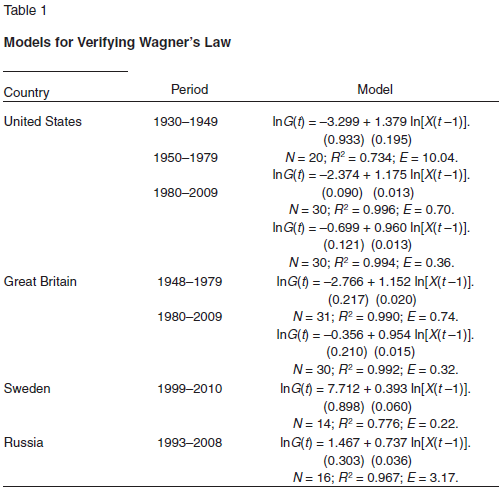
The only difference between model (2) and the classical Peacock–Wiseman model is that in model (2) GDP is taken into account with a one–year lag (t – time, year). The parameters β and θ require identification, with m=eβ. Despite its simplicity, relationship (2) quite successfully describes the actual processes and is fairly universal [8]. If the elasticity θ>1, then Wagner’s law is fulfilled; if θ ≤ 1, then Wagner’s law is violated (for a more detailed analysis of Wagner’s law, see our previous work [9]).
For the four countries in question, econometric relationships were obtained on the basis of official statistical data [10] and are given in Table 1. The following notations are used in the models: N is the number of observations; R2 is the coefficient of determination; and E is the mean error of approximation (in percent of the actual value). The values of the standard errors are indicated in parentheses under the regression coefficients. All of the models passed the basic statistical tests.
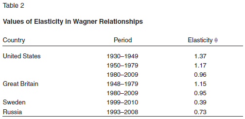
Based on the models that were constructed, we determined the values of the elasticities θ for each of the countries. The results are given in Table 2.
The results of the calculations enable us to draw a number of important conclusions.
First of all, it seems that Wagner’s law is no longer relevant. This is true both of classical capitalist countries (the United States and Great Britain), countries with strong social models (Sweden), and countries with transition economies (Russia). Recall that, according to Durevall and Henrekson’s calculations, Wagner’s law was in effect in Great Britain throughout the period from the 1960s until the end of the 1970s, but it lost force after that [11]. This claim fully agrees with our results, and our conclusions also coincide with those that Durevall and Henrekson reached in regard to Sweden.
Another important conclusion is the clear weakening trend of Wagner’s law. This trend can be seen most distinctly in the U.S. economy θ=1, and thereby overturned Wagner’s law. Great Britain has also been characterized by analogous processes. In any case, the global direction of economic systems’ evolution is obviously toward suppression of Wagner’s law.
Another interesting fact should be noted: over time elasticity θ is decreasing, against the background of increasingly accurate approximation of the relationship (2). For example, in the United States and Great Britain, the value of the error of approximation E has fallen sharply. In other words, the more Wagner’s law weakens, the more the connection between government spending and GDP stands out. At first glance, such a situation may seem paradoxical, but, there is a quite natural explanation for this. The point is that the faster the budget is inflated, the less stable it is and the less reliable the averaged relationship between it and the trajectory of GDP becomes. An increase in parameter θ actually causes a sharp deviation from the GDP trend and makes a high correlation between government spending and GDP problematic.
Thus, many countries have made the transition to a different mode of functioning, in which economic growth no longer leads to an increase in the percentage of government spending in GDP. To all appearances, this is because many countries have come up against some factors that limit the growth of this parameter. One is the Armey–Rahn curve, in relation to which there are also many questions.
Identification of the Armey–Rahn curve
According to contemporary ideas, the Armey–Rahn curve defines a parabolic relationship between the growth rate of GDP (λ=ΔX/X) and the percentage of government spending in GDP (g=G/X) (the curve is presented in this form, for example, by Daniel Mitchell) [12]. So we are talking about a curve λ=λ(g). The maximum point on this curve is called the Scully point, and the conditions dλ/dg =0 and d2λ/dg2<0 are fulfilled for it. Beyond this point, growth in the share of government spending begins to restrain economic growth in the sense of lowering its rate.
We believe that the simplest parabolic function x = x(g) can serve as the basic analytical construct of the Armey–Rahn curve, as was done previously [13]:
x = αg + bg2 (3)
where x=1+λ is the growth rate of GDP; and α and b are parameters that can be estimated econometrically.
The difference between model (3) and the traditional Armey–Rahn curve is that on the left side of (3) we have the GDP growth rate, rather than its rate of increment. This form of the relationship is determined by technical considerations. Jumping ahead, we note that the testing of model (3) showed its universality against a background of good statistical characteristics, while introducing a “pure” parameter λ on the left side immediately broke the relationships that were revealed. In all likelihood, this effect is due to the occurrence of high volatility of the left side of the model due to the presence in it of quantities with different signs. The addition of 1 to λ not only resulted in all of the dependent variables in model (3) being positive but also to averaging of their scale. Econometric models (3) for various countries are given in Table 3.
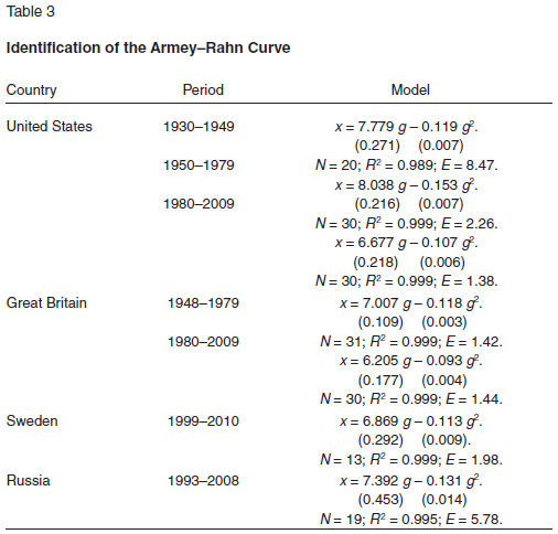
The calculations show that the Armey–Rahn curve takes place in its refined form in all of the countries in question. And the accuracy of the models increases with time, as in the case of Wagner’s law.
The main advantage of the models that were constructed consists in their simplicity and universal parabolic form. This makes it possible to estimate a number of important indicators of the Armey–Rahn curve.
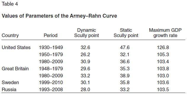
The first one is the dynamic Scully point (g*), which corresponds to the maximum on the dynamic Armey–Rahn curve. Here we should note that all of the models we constructed are dynamic Armey–Rahn curves, since the GDP growth rate appears on their left side, rather than the absolute value. Then the dynamic Scully point g* satisfies the conditions dx/dg=0 and d2x/dg2<0. For model (3), this point has the form:
g* = –α/2b (4)
Second is the maximum growth rate of GDP (x*), which can be achieved at the maximum point of the dynamic Armey–Rahn curve: x*=x(g*). This quantity indicates some potential possibilities of the national economy in the most favorable government spending conditions. For model (3), this point has the form:
x* = –α2/4b (5)
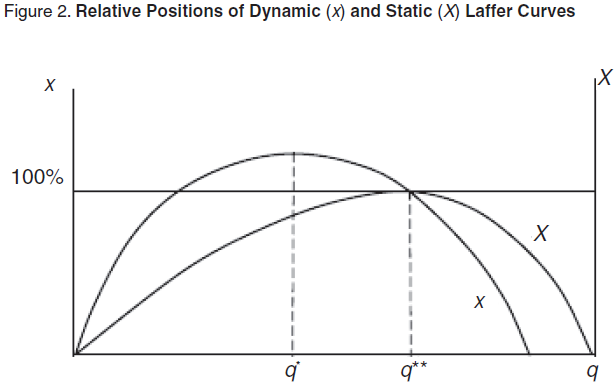
Third is the static Scully point (g**), which corresponds to the maximum on the static Armey–Rahn curve. To find this point, we have to take into account the fact that the absolute value of GDP starts to diminish only after x, passing the maximum point on the dynamic Armey–Rahn curve, drops below the line x=1 (x=100 percent). Consequently, the static Armey–Rahn curve is somewhat deformed in relation to the dynamic curve, and its hump will be shifted to the right on the g scale. Then the static Scully point g** satisfies the conditions x=1 and g*=g**. In other words, the static Scully point is always greater than its dynamic analogue. For model (3), this point is found from the quadratic equation bg2+αg–1=0. Of the two points that solve the equation, the static Scully point will be the greater one, which is farther to the right on the g scale. For model (3) this point has the form:
.png) (6)
(6)
The values of these three indicators are given in Table 4.
The estimates obtained indicate at least three interesting facts.
The first fact is that the values of the static Scully points are five to six percentage points greater, on average, than the values of the dynamic Scully points. This interval shows the scale of government regulation that separates a policy of achieving the maximum economic growth rate from a policy of falling into a recession. This indicates that the margin between a policy that encourages growth and a policy that restrains growth is not so broad. Excessive pumping up of government spending may imperceptibly lead to depression. If it is taken into account that the actual parameters of the economy are generally higher than the values of the dynamic Scully point, this course of events becomes even more likely.
The second fact involves the fairly clear drift of the Scully point in the direction of an increase. The evolution of economic systems toward bigger budgets and business’s adaptation to this trend have an effect here. If economic development is interrupted by some exogenous circumstances that require mobilization of the country’s resources, then the Scully point may increase sharply. In particular, such a situation took place in the United States in 1929–49, when the Great Depression and World War II took place.
The third fact is that the value of the maximum growth rate x* is decreasing. It seems that what we have here is a gradual exhaustion of the stimulating potential of budget policy. Calculations shows that even ideal fine-tuning of budget spending can provide for an annual economic growth rate of only 3 percent. National economies are unlikely to surpass this limit without some exogenous and particularly favorable circumstances. Meanwhile, up until the second half of the twentieth century the United States was capable of a truly fantastic growth rate (26 percent), thanks to correct manipulation of the parameter g.
Identification of the Laffer production curve
As we have already noted, budget spending policy is preceded by fiscal policy, which is aimed at replenishing the government’s coffers. Here the relationship between GDP and the tax burden is reflected by the so–called Laffer production curve. In its canonical form, this curve defines a parabolic relationship between the amount of GDP (X) and the tax burden, which is calculated in the form of the percentage of government (tax) revenues in GDP (q=T/X, where T is the budget’s tax revenues). Thus, we are talking about the curve X=X(q).
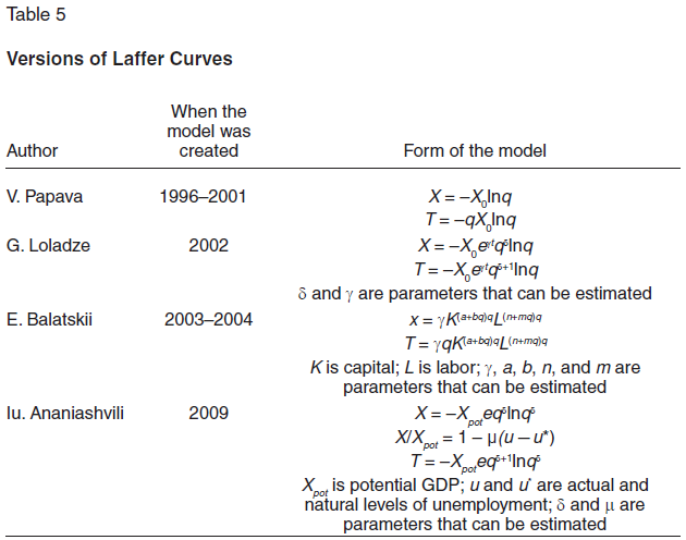
A great many studies, of both a theoretical and an empirical nature, have been devoted to the Laffer curve now. Here we point out, first of all, the work of Arthur Laffer himself [14]. The introduction of the concept of Laffer points of the first and second kind was an interesting continuation of the doctrine of the Laffer curve [15]. These points were later subjected to scrupulous econometric identification. For the most part, this was done using a static, three-factor relationship of the type X = X(K, L, q), where GDP (X) was considered to be dependent on the number of people employed (L), the amount of fixed capital (K), and the tax burden (q) [16]. However, this approach proved to be fairly complicated and had a number of shortcomings [17]. In 2010, Iurii Ananiashvili and Vladimer Papava tried to construct a synthetic system that would accommodate both demand theory based on the multiplier concept and supply theory, including the concept of the Laffer curve [18]. In addition, in 2001, Papava suggested two important theoretical versions of the Laffer curve [19].
In parallel with this, there have been periodic attempts to construct alternative algorithms for computing Laffer points. Economists of the Georgian school have made a big contribution in this direction. For example, in 1996, Papava suggested that fiscal effects could be described with a single-factor entropy function X = X(q), which mostly served for theoretical illustration of supply economics [20]. Later, in 2002, starting from this analytical concept, G.Loladze suggested a generalized entropy function, the parameters of which can be estimated econometrically [21]. In 2009, Ananiashvili took another step in generalizing the entropy function and supplemented it with an algorithm for estimating the parameters using an equation that describes Okun’s law [22]. All of these models are shown in Table 5.
However, all of these approaches were based on the methodology of static functions, which created serious computational difficulties and led to highly doubtful estimates. In our opinion, this was because all of these econometric models contained variables of different dimensions and, consequently, of different scales. There are technical difficulties associated with calibrating such relationships, which are manifested in overestimated or underestimated fiscal parameters. In this regard, the relationship that we have established for describing the Armey–Rahn curve provides the key to a different way of determining the Laffer points. If we transfer model (3) to the case of dependence of the GDP growth rate on the tax burden, we get a description of the dynamic Laffer curve:
x = α*q + b*q2 (7)
where a* and b* are parameters that can be estimated.
In this case, the quantities on the right and left sides of the regression are commensurable and of the same order, calculated in percent. Calculations show that relationship (7) is universal and provides a good approximation of the process that is being modeled (Table 6).
.png)
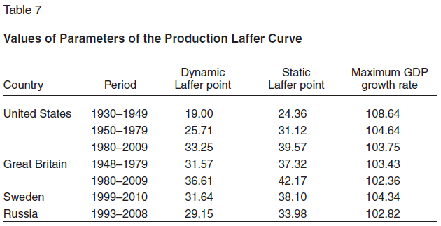
As it turns out, the dynamic Laffer curve (7) is easily determined according to statistical data, in contrast to the static Laffer curve. At the same time, the presence of model (7) makes it possible to automatically obtain three indicators, by analogy with the Armey–Rahn curve. They are the dynamic Laffer point (q*), the static Laffer point (q**), and the maximum economic growth rate (x*) (Table 7).
The estimates allow us to draw conclusions analogous to those drawn in calculating the Scully points. We discuss them briefly.
First, the static Laffer points are five to six percentage points greater than the dynamics ones, on average.
Second, with time the Laffer point drifts in the direction of an increase. Even the period in which the Great Depression and World War II took place did not change this trend. This shows a striking contrast with the Scully point. Consequently, extreme economic circumstances in the form of crises and wars generally increase the efficiency of government spending but do not affect the psychology of business in the sense of its tolerance of the tax burden.
Third, the value of the maximum growth rate x* is decreasing. Here we have a gradual exhaustion of the stimulating potential of the government’s fiscal tools.
Note the following point in particular. As we have already said, identifying static Laffer points is a very laborious procedure, while finding dynamic Laffer points turns out to be an almost trivial operation. Furthermore, the parabolic relationship (7) is extremely convenient for all subsequent computations. At the same time, the transition from a dynamic to a static Laffer point is elementary, which makes it possible to estimate a static Laffer point by a two-step procedure that is notable for its simplicity and clarity. This algorithm was largely unexpected for the authors, in spite of how obvious it is.
The suggested new methodology for estimating the Laffer point is nontrivial for previous studies. According to this methodology, a static Laffer curve is actually re-created according to an available dynamic Laffer curve (Figure 2).
We will immediately point out that, according to the established terminology, point q* is the Laffer point of the first kind. Analysis of the Laffer point of the second kind is also possible, but it seems less substantive. For example, from the relationship T=qX it is easy to find that 1+ΔT/T=kx, and the Laffer point of the second kind is found from the equation bg2+αg–1/k=0, where k is an index of growth of the tax burden (k=1+Δq/q). If k>1, which corresponds to the situation when the tax burden is growing, with movement to the right on the tax scale, then the Laffer point of the second kind will always be greater than the Laffer point of the first kind. This directly follows from the equation for the Laffer point of the second kind (q***):
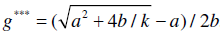 (8)
(8)
However, in our opinion, we can limit our analysis, by and large, to the Laffer point of the first kind. In connection with this, note that some researchers think that the Laffer point of the second kind is not at all suitable as a serious reference point for fine–tuning fiscal policy [23]. For example, I. Maiburov believes that the optimal tax burden should be no greater than the Laffer point of the first kind [24].
Generalizing everything all that has been said, we can draw the following conclusions.
First, fiscal analysis should be expanded to cover three indicators: the dynamic Laffer point (q*) and static Laffer point of the first kind (q**), and the static Laffer point of the second kind (q***). However, only the first two points are key for developing fiscal policy; the Laffer point of the second kind should be used mostly for in–depth analysis of the tax system’s efficiency.
Second, estimation of the dynamic Laffer point (q*) and the static Laffer point of the first kind (q**) should be done using the simple model (7). Use of this simple parabolic relationship makes it possible to avoid a great many technical problems in maintaining methodological unity of the analysis of fiscal effects.
Relative positions of the Scully and Laffer points
As we have said, the Scully points set a serious barrier to economic growth. However, the Laffer points also put up a similar barrier. This raises a reasonable question: which of these two barriers is more active and inflexible?
To answer this question, we calculate two simple indicators: the dynamic optimal budget deficit (ρ*) and the static optimal budget deficit (ρ**):
ρ* = g* – q* (9)
ρ** = g** – q** (10)
When ρ* > 0, the economic system runs up against the Laffer point sooner, while the Scully point is dormant; otherwise the Scully point, on the contrary, takes effect sooner than the Laffer point. Analogous logic applies to the parameter ρ**.
Estimates of indicators (9) and (10) are given in Table 8, based on which we can draw the following conclusions.
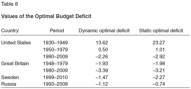
First, there is no clear pattern in the relative locations of the Laffer curve and the Armey–Rahn curve. Experience shows that in the United States up to the 1980s the hump of the Armey–Rahn curve was to the right of the hump of the Laffer curve, which contradicts the typical diagram drawn by Lawrence Hunter [25]. However, after the 1980s the humps on the Laffer production curve and the Armey–Rahn curve changed places. All of the countries under consideration have recently been tending toward a surplus budget management regime. It seems that this shift in policy indicates the growth of objective constraints on generation of revenue and government expenditure.
Second, Almost all countries are now conducting a surplus budget policy, with a relatively small safety cushion of 1–3 percent of GDP. It seems that the era of deficit budgets has passed and contradicts the logic of the current economic growth regime. However, paradoxical it may be, the Armey–Rahn curve is more important today than the Laffer curve is.
Can a substantive interpretation of this fact be given?
In our opinion, the situation is as follows. Growth of the tax burden suppresses business and investment activity. The desire to make extra efforts and struggle for a low profit margin fades away. However, growth of the scale of government spending means centralized support of a certain part of the economy, which makes market competition less intense and transfers it to the field of so–called rent–seeking [26], which consists in lobbying for government purchases. Moreover, private investments are displaced by government investments, which lowers the investment activity of businesses. The presence of a rent component in government subsidies that are received gradually leads to a decline in economic efficiency and the economic growth rate. Thus, growth of the tax burden and the scale of government spending leads to the same result via different mechanisms.
And another question arises: Why is a change of regimes occurring, with recombination of the relative positions of the Armey–Rahn curve and the Laffer curve?
In our opinion, the answer to this question has an evolutionary sound. As the tax burden grows, business adapts to it and demonstrates greater tolerance. Growth of fiscal tolerance leads to deformation of the Laffer production curve and a gradual shift of the Laffer point to the right. Along with this, growth in the scale of government participation in the economy has enormous prospects in the initial stage, on the strength of the undeveloped market for public goods. However, as this market is developed, saturation of it occurs, with a corresponding decline in the efficiency of government investments. The decrease in the return on government spending is equivalent to deformation of the Armey–Rahn curve, with a shift of the Scully point to the left. The development of these two processes in different directions can lead to a switch in the positions of the Armey–Rahn curve and the Laffer curve, which we can see on the example of the United States (Table 8).
Thus, the transposition of the Scully and Laffer points is associated with different speeds of the system’s adaptation to the different mechanisms. The rate of the system’s adaptation to the tax burden, which is reinforced by technological innovations, is greater than the rate of adaptation to saturation of the market for public goods and mastery of administrative methods of competition.
As for practical conclusions, we can state that, since the Scully point is now the active limit on economic growth, the development of budget policy should be guided primarily by that point. This means that the actual values of the share of government spending (g) should lie in the interval g*≤g≤g**. This principle should be reinforced by a milder limit for the tax burden: q*≤q≤q**.
Notes
1. See S.Lamartina and A.Zaghini, “Increasing Public Expenditures: Wagner’s Law in OECD Countries,” Unversidad de Salamanca, 2008, http://campus.usal.es/~XVEEP/PAPERS/J1S6/XVEEP-29 percent20LAMARTINA-ZAGHINI.pdf.
2. See D.Durevall and M.Henrekson, “The Futile Quest for a Grand Explanation of Long-Run Government Expenditure,” Research Institute of Industrial Economics, IFN Working Paper, no. 818 (2010).
3. See M.A.Babatunde, “A Bound Testing Analysis of Wagner’s Law in Nigeria: 1970–2006,” paper presented at the African Econometric Society, Thirteenth Annual Conference on Econometric Modeling in Africa, July 9–11, 2008, University of Pretoria, South Africa; available at www.africametrics.org/documents/conference08/day1/session2/babatunde.pdf.
4. See C.Ighodaro and D.Oriakhi, “Does the Relationship between Government Expenditure and Economic Growth Follow Wagner’s Law in Nigeria?” Annals of the University of Petro ani, Economics, 2010, no. 10(2).
5. See S.Verma and R.Arora, “Does the Indian Economy Support Wagner’s Law? An Econometric Analysis,” Eurasian Journal of Business and Economics, 2010, no. 3(5).
6. See E.V.Balatskii [Balatsky], “Zakon Vagnera, krivaia Armi–Rana i paraodks bogatstva,” Obshchestvo i ekonomiki, 2010, no. 9. [Translated in this issue, pp. 40–54].
7. See A.Peacock and J.Wiseman, The Growth of Public Expenditure in the United Kingdom (Cambridge: NBER and Princeton: Princeton University Press, 1961).
8. Note that in “Zakon Vagnera, krivaia Armi–Rana i paraodks bogatstva,” we used a relationship without the absolute term (β=0). Such formalization leads to a system error, since the inequality θ<1 always takes place.
9. See Balatskii, “Zakon Vagnera, krivaia Armi–Rana i paraodks bogatstva.”
10. See Statistical Yearbook of Sweden, 2011, www.scb.se; Federal’naia sluzhba gosudarstvennoi statistiki, www.gks.ru; UK National Statistics, www.statistics.gov.uk; Bureau of Economic Analysis, www.bea.gov.
11. See Durevall and Henrekson, “The Futile Quest for a Grand Explanation of Long-Run Government Expenditure.”
12. See D.Mitchell, “The Impact of Government Spending on Economic Growth,” Heritage Foundation, 2005, www.heritage.org/Research/Reports/2005/03/The-Impact-of-Government-Spending-on-Economic-Growth/.
13. See Balatskii, “Zakon Vagnera, krivaia Armi–Rana i paraodks bogatstva.”
14. See A.B.Laffer, “The Laffer Curve: Past, Present and Future,” Heritage Foundation Backgrounder, no. 1765, June 1, 2004, www.heritage.org/research/taxes/upload/64214_1.pdf.
15. See E.V.Balatskii, “Analiz vliianiia nalogovoi nagruzki na ekonomicheskii rost s pomoshch’iu proizvodstenno-institutsional’nykh funktsii,” Problemy prognozirovaniia, 2003, no.2; idem, “Otsenka vliianiia nalogovykh instrumentov na ekonomicheskii rost,” Problemy prognozirovaniia, 2004, no.4.
16. Balatskii, “Otsenka vliianiia nalogovykh instrumentov na ekonomicheskii rost”; A.G.Gusev, “Vliianie fiskal’nykh instrumentov na ekonomicheskii rost: metod makroanaliza,” Candidate of Economic Sciences dissertation (Moscow: IMEI, 2003).
17. See Iu.Ananiashvili and V.Papava, Nalogi i makroekonomicheskoe ravnovesie: laffero–keinsianskii sintez (Stockholm: Izdatel’skii dom CA&CC Press, 2010).
18. See ibid.; Iu.Sh.Ananiashvili and V.G.Papava, “Laffero–keinsianskii sintez i makroekonomicheskoe ravnovesie,” Obshchestvo i ekonomiki, 2010, no.9.
19. See V.G.Papava, “Lafferov effekt s posledeistviem,” Mirovaia ekonomiki i mezhdunarodnye otnosheniia, 2001, no. 7; V.Papava, “On the Laffer Effect in Post–Communist Economies (On the Basis of the Observation of Russian Literature),” Problems of Economic Transition, 2002, vol. 45, no. 7, pp. 63–81.
20. See V.Papava, “The Georgian Economy: from ‘Shock Therapy’ to “Social Promotion,’” Communist Economies and Economic Transformation, 1996, vol. 8, no.8.
21. See G.O.Loladze, “O nekotorykh aspektakh krivoi Laffera,” Makro mikro ekonomiki, 2002, no.9 (in Georgian).
22. See Iu.Ananiashvili, “Vliianie nalogov na sovokupnoe predlozhenie,” Ekonomika da biznesi, 2009, no.1 (in Georgian); idem, “Modeli otsenki fiskal’nykh parametrov,” Ekonomisti, 2009, no.1 (in Georgian).
23. See I.A.Maiburov, Teoriia nalogooblozheniia. Prodvinutyi kurs: uchebnik dlia magistrantov (Moscow: IuNITI-DANA, 2011), p. 331.
24. See I.A.Maiburov, ed., Nalogovaia politika. Teoriia i praktika: uchebnik dlia magistrantov (Moscow: IuNITI–DANA, 2010), p. 103.
25. See L.A.Hunter, “The Leviathan Project,” The Institute for Social Choice and Individual Values, 2008, www.socialsecurityinstitute.com/uploads/File/The–Leviathon–Project–Web.pdf.
Translated by James E. Walker
Official link to the article:
Balatsky E.V., Ekimova N.A. Fiscal Policy and Economic Growth// Problems of Economic Transition, vol.54, no.12, 2012, pp. 55–70.