Introduction
The establishment of market economy in Russia led to the predictable income stratification of society. Social conflicts today are becoming more intense and attract a lot of attention. At the same time, the introduction of international sanctions worsened the situation with the country’s budgetary revenues. Both problems could, at least partially, be solved by the introduction of a progressive income tax scale (IT), so this issue has been prominent in the political discourse of the past two years.
The analysis shows that the society is divided into two camps on the issue of introducing the progressive personal income tax (PPIT). On the one hand, the State Duma (SD) receives constant proposals to introduce this fiscal instrument, on the other hand – the Government of the RF unfailingly refuses to support these initiatives. Thus, in 2017 three political fractions supported the draft law to introduce a progressive individual income tax scale: the Communist Party of the Russian Federation (CPRF), the Liberal–Democratic Party of Russia (LDPR) and the Party “Just Russia” (PJR). The draft laws proposed by these parties differed only in details – in tax rates and the gradation of income. However, the Government of the RF did not support these initiatives; in the end, the SD of the RF rejected these draft laws. It should be mentioned that “Just Russia” submitted drafts for discussion in the SD of the RF over ten times, with invariably negative results. In this case, it is impossible to overlook the fact that all projects to introduce the PPIT were always approved by the Parliament of the Kabardino–Balkar Republic. Thus, it is possible to state that there is, so far, no political consensus in Russian society regarding the PPIT. The situation worsened in 2018, after the pension reform had been initiated. From that moment, it became clear that the Government of the RF chooses to solve budgetary problems at the expense of poor, rather than rich, members of the society.
At present it is possible to single out four projects of the income tax reform – those of three political fractions (PJR, LDPR and CPRF) supporting the introduction of the progressive scale of income tax, and the Government of the Russian Federation (GFR) that proposes to preserve a flat scale while simultaneously raising its rate from 13% to 15%. Each of the scenarios is characterized by different risks of non–fulfillment. The goal of this article is to develop a standard methodology for the economic evaluation of tax reform projects and the selection of the most appropriate one. Three groups of risks will be taken into consideration – fiscal (additional revenue for the budget), social (changing the income disparity), and behavioral (the degree of project feasibility). The calculations should illustrate the functionality of the developed methodology; they could be used in the future for the examination of any projects of the IT reform.
For the future analysis of the tax reform problems it is important to remember that we are going to discuss the PIT, although this tax is not used in Russia and is substituted by its distant equivalent – the income tax of natural persons (ITNP). The difference between them lies in the fact that PIT takes into account the per capita family tax, while ITNP is limited to the income of a specific person; in other aspects PIT and ITNP are functionally identical. To ensure a correct transition from the Russian ITNP to the international standard of PIT, the authors will carry out special calculations aimed at making them comparable.
Analytical overview of the problem
There are numerous publications discussing different aspects of social inequality and income tax; however, for the purposes of this article, it will be sufficient to point out a number of key ideas to fit in the general trend of the existing research.
Primarily, it should be noted that in most countries where the share of PIT in the budgetary revenue is low, this situation is connected with the low income level in general and the level of wages in particular [1, 2, 3, 4]. Although the incomes of people in Russia have grown considerably in the last two decades, they still have not reached the level at which the PIT becomes the fiscal dominant of the budgetary system. From this point of view, no changes of the system of PIT in Russia will lead to a radical increase of its role, and this factor should be taken into consideration while reforming the Russian tax system.
It should be borne in mind that the transition of Russia to a flat scale of PIT was happening simultaneously with similar reforms in other countries, for example, Sweden. Such political decisions were mainly connected with the understanding that, due to a large number of special regimes and benefits, the PIT had probably not completely lost, but had still greatly decreased its redistribution functions and progressive character [5, 6, 7]. Econometric calculations in the following years showed that the PIT is mainly oriented at leveling the wages, while its potential for the redistribution of taxable incomes of high-income groups is, on the whole, low [8].
An important milestone in the research of the PIT were the models of individual tax evasion, where the function of utility depended on the size of the individual’s “wealth”. One of the first such models was proposed as far back as 1972 [9], followed by a stream of publications that studied its specific aspects [10, 11]. With reference to Russia, it was shown that a modest role of the PIT in the tax system was mainly connected with various tax evasion mechanisms used by high income taxpayers [8].
The past decade in Russia has been characterized by an accent on the analytical description of the fiscal effects and the effects of social inequality. Thus, for example, the distribution of income in groups of population was approximated using the Verhulst differential equation, which made it possible to obtain an analytical expression for the assets ratios, Gini index and the coefficient of specific polar incomes, as well as to determine that there were not significant changes in the structure of income distribution in 2009–2015 [12]. An attempt was made to model the income distribution function in Russia with the use of the two–parameter long–normal distribution, which allowed to evaluate the assets ratio in 1998 at the level of 17.6 for the country as a whole, while for Moscow it was at the breathtakingly high level of 46.0 [13].
More advanced research of the recent years has been mainly aimed at modeling the progressive scale of the PIT. This was greatly predetermined by the fact that the modern theory of optimal income taxation, which goes back to the works of J.Mirrlees [14], does not provide any comprehensive answers to the question of the optimal progression degree for the PIT scale or the size of top rates and the range of their variations. Besides, the obtained analytical results are very sensitive to the initial suppositions and assumptions, which in their turn, according to some researchers, are themselves weakly grounded and insufficiently substantiated [15]. In this connection, a game model of constructing the progressive scale of PIT was put forward in 2011, it used the differential “coupling equation” as the main condition for the model’s solution [16]. The obtained results made it possible to reduce the problem of selecting the top rates of the PIT and the grades of the scale to the problem of choosing five entrance parameters for this model, which could be easily determined on the basis of statistical data. For the case of long-normal distribution of income, the progressive scale of PIT was determined as fractions of the mathematical expectation, and the percentage (effect) of this type of tax from the aggregate tax revenue was expressed through the parameter of dispersion in the distribution [17].
Theoretical research in the sphere of taxation made it possible to determine that a small change of prices caused by the introduction of the PIT, leads to a considerable change (deterioration) of the standard of living [18]. Further modeling of the economic effects from the introduction of the PPIT allowed to derive the function of the redistribution of the tax burden and to compare multiple variants of the non–linear tax [19].
As for the flat PIT scale, it was shown that the instruments ensuring its progressiveness are the standard benefits. However, due to the incomplete and untimely indexation of the ITNP benefits and the abolition of the standard benefit, the progressiveness of the PIT decreased in the decade following its introduction, and the emerging effect of “cold progression” lead to the additional taxing of the sums which should have been removed from the taxable base on the grounds of the social function of the taxes [20].
In recent years, some ultramodern instrumental approaches to studying the income tax phenomenon have been developed. One of them is the analysis of the dynamics of income tax evasion based on the standard model of statistical mechanics, namely, the Ising model of ferromagnetism [21]. This approach within the framework of econophysics makes it possible to examine a heterogeneous society whose agents are characterized by a certain social temperature and connection with the external fields that govern their behavior. This new approach to modeling allows to analyze big communities consisting of at least four different interacting types of agents.
Research based on the agent–oriented models and aimed at studying behavioral and social aspects of taxation has also recently gained popularity. Thus, there are works aimed at determining the role of professional affiliation in the observance of tax legislation (tax discipline) and the conditions of auditing (checking) a fixed number of taxpayers for each type of professions [22].
There are also some model applications of the imitation type used to assess different variants of income tax reform. One of them is the MIKMOD–ESt model that belongs to the class of the so–called micro–simulation models [23]. This model was developed and is used by the German Federal Ministry of Finance to evaluate different proposals regarding the reform of the income tax of individuals. Its advantage is the total inclusion of all taxpayers with the above–threshold income, which makes it possible to conduct calculation experiments even for the most selective reforms; its drawback is the absence of information necessary for modeling the behavioral reactions of taxpayers to the changes in taxation.
Various models of the progressive scale of income tax based on the principle of multiplicator–accelerator remain relevant. Thus, it is believed that in the cases on non–linear progressive taxation the increase of tax rates could destabilize the economic growth [24]. Such models let the policymaker obtain the conditions for a stable growth as a “corridor” of parameters’ values for the fiscal regime of stability.
Another research area with numerous publications is connected with the risks caused by tax reforms. Currently there are various definitions of this concept, which are studied in detail in the following publications [25, 26]. In spite of the multitude of approaches to their interpretation, all authors agree that tax risks are caused by the uncertainty of both external and internal environment, they are connected with the threat of financial and other losses for the state and the taxpayers, they have a negative character and are rather hard to identify and to assess [27].
The causes of uncertainty include the following categories of risks [28]: information risks connected with different interpretations of legislative acts; risks of the process that emerge when the tax liabilities are carried out (managerial mistakes, drawbacks of the document flow, portfolio risks, etc.); risks of the environment – the consequence of uncertainties in the enforcement of tax legislation; reputational risks – risks of hurting the reputation of the company. Some authors extend this list and add risks of financial accounting and management [29]. Besides, many researchers believe that tax risks emerge as a consequence of a great tax burden when taxpayers try to evade their tax obligations and thus contribute to the growth of the shadow economy [30, 31]. This is the key argument of the advocates of preserving the flat scale of the ITNP when discussing the choice of the taxation system for Russia. Specifically, the Government of the RF has rejected all the analyzed draft laws on changing the taxation system on the grounds of the experience of 1992–2000 when a progressive scale of tax rates was used in Russia. The negative effects include the difficulties of administrating and the desire of taxpayers (both employers and employees) to reduce the tax burden through the minimization of the paid (received) income. Besides, it states that the introduction of a flat ITNP scale in 2001 contributed not only to the increase of tax revenue, but also to the stabilization of tax collection.
The position of the authors is closest to the views presented in [32], which examines the possibility of restoring the PIT in Russia and offers a quantitative evaluation of the possible results of this step for the three hypothetical scenarios of the reform. In particular, the author shows the drawbacks of the existing statistical information and models the income distribution curve. The calculations of the budgetary revenue and the decile coefficient showed that none of the three scenarios of introducing the PIT ensures a considerable reduction of the decile coefficient, which supports the conclusion of previous research regarding a weak redistribution function of the PIT.
The article [33] studies the influence of the election cycles on the Russian tax system. Specifically, the authors showed that the tax burden on the main elements of GDP increases during the first years of the political cycle, and decreases during its last years. Thus, in the pre–election period the nominal tax burden on the economy is constantly decreasing, in the election year and the following year of the election cycle the effective rates of revenue, consumption and labor all rise; these effective tax rates go down in the following years. Consequently, the implementation of tax reforms critically depends on their starting date with reference to the beginning of the election cycle.
In the following sections of the articles the authors will try to unite some of the abovementioned aspects of taxation within the framework of a single analytical scheme which would combine real projected parameters of reforms and the model constructions.
The three–parameter model of the progressive personal income tax
The authors use the three–parameter model to evaluate the expediency of introducing the PPIT. In this case, the model scheme will take into account three key parameters – social (assets ratio), fiscal (growth of tax revenue), and behavioral (the degree of project feasibility). It is expected that the introduction of the PPIT should lead to a reduction in the assets ratio and a growth in tax revenue while taking into consideration the risk of failing to implement the reform project. The main idea of this scheme is that the calculations should simultaneously take into account three consequences of introducing a progressive scale of the PIT. Let us take a closer look at all the dependences used later on.
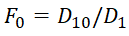
The initial value of the assets ratio, i.e. before a progressive scale of the PIT is introduced, is calculated in the trivial way:
 (1)
(1)
where D1 and D10 – the income of the 1st and the 10th decile groups.
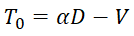
The initial value of tax revenues from PIT could be evaluated by a simplified equation:
 (2)
(2)
where D – the population’s aggregate income; α – basic rate of PIT [1]; V – tax benefits.
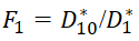
Then the assets ratio after the introduction of the PPIT is calculated as:
 (3)
(3)
where D*1, D*10 – the aggregate income of the 1st and the 10th decile groups after the introduction of the progressive scale of the PIT.
In the simplest case it is possible to neglect the tax benefits (V=0). Then the whole effect of the tax reform is determined by a new value (after the introduction of the PPIT) of the income of the 10th decile group D*10:
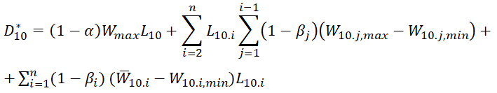
(4)
where Wmax – the maximum income for the basic rate of taxation (α); L10 – the size of the 10th decile group; L10,i – the size of the i subgroup of the 10th decile group; βi and βj – the tax rate of the i and the j subgroups of the 10th decile group, correspondingly; W10,j,max – the upper income threshold of the j subgroup of the 10th decile group; W10,i,min and W10,j,min – the lower income threshold of the i and the j subgroups of the 10th decile group, correspondingly;  – the average income of the i subgroup of the 10th decile group;
  ; n=5.
The volume of tax revenues from the PIT after the introduction of the progressive scale is calculated according to the formula:

(5)
For further analysis, it is necessary to evaluate the two abovementioned parameters: the change of the assets ratio after the introduction of the progressive scale
 (6)
(6)
and the absolute and the relative change of tax revenues regarding the PIT
 (7)
(7)
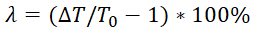 (8)
(8)
To compare different scenarios of tax reform, the criteria (6) and (8) can be aggregated into one with the help of mass coefficients ζ and 1–ζ. Then it is possible to use the simplest convolution equation:
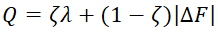 (9)
(9)
where ζ – mass coefficient.
To compare the scenarios of the introduction of the progressive scale with the scenario of changing the flat scale, it is sufficient to evaluate the tax revenues for the second case according to the equation:
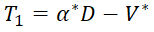 (10)
(10)
where α*– the new flat rate of the PIT.
However, even the combination of the fiscal and the social effects does not make it possible to determine the best scenario of the tax reform. The matter is, each of the examined four scenarios is characterized by one more important parameter – risk (R). Risk in this case is understood as the probability that the projected scenario will not in practice lead to the planned effect. In this sense, the integral effect Q acts as the potential effect that could be reached fully or partially in the implementation of the project. Thus, to make a decision regarding the expediency of a project, it is necessary to have one more project feature – the size of the risk of its fulfillment/non–fulfillment. The combination of the potential effect with the rate of risk makes it possible to assess the factual (real) effect.
At the qualitative level it is evident that the projects of the PJR and the GRF include a low risk, the CPRF project – a medium risk, and the LDPR project – a high risk. However, this rough estimate of risk does not allow for a correct comparison of these projects, which differ considerably in the size of their potential effect. To do this, a concrete index of risk R is needed, with its specific quantitative value. This index could be used to range the projects of the PIT reforms on the basis of the aggregate criteria of result E.
Theoretically, the aggregate criterion E could be set in the additive and the multiplicative form. In instrumental terms, the multiplicative criterion is preferable and could be written as following:
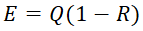 (11)
(11)
where the potential fiscal–social effect Q is corrected by the factor of reliability D=1–R, which is the measure reverse to the risk R. It is easy to see that the reliability coefficient D acts as some kind of efficiency coefficient (EC). Thus, the equation (11) includes a maximally transparent interpretation of the modeled process: the final effect is the value of the potential effect with the assessment of the EC of the examined reform scenario.
The presented equations make it possible to maximally correctly determine the social and fiscal results of both the scenarios with different progressive scales of the PIT and the scenarios of simply changing the flat scale.
Initial data for modeling
All macroeconomic evaluations of tax effects, as a rule, are relative and do not claim to be highly precise. However, our task in this case is to do maximally accurate calculations to understand the comparative effect of different scales – the flat one and the progressive one. To achieve this, it is necessary to prepare the initial data for macro–calculations very thoroughly. Below we present the algorithm of calibrating the statistical aggregates and their “corrected” values that let obtain non-contradictory results in the future.
The first set is data on the distribution of the population’s incomes broken into groups, each of which comprises 10% (Table 1). To balance all values, the last column of Table 1 is calculated as the product of columns 3 and 4, which led to a small error compared with the Rosstat data.
Table 1
The distribution of monetary income by 10% groups of population in 2016
|
Income groups |
Share of the group in the total volume of monetary income of population, % [2] |
Size of the group, th. people |
Average per capital monetary income, RUB per month [3] |
Monetary income of the group in 2016, RUB |
|
First |
1.9 |
14 680 400 |
5 983 |
1 053 993 998 400 |
|
Second |
3.4 |
14 680 400 |
10 368 |
1 826 476 646 400 |
|
Third |
4.5 |
14 680 400 |
13 704 |
2 414 162 419 200 |
|
Fourth |
5.6 |
14 680 400 |
17 107 |
3 013 651 233 600 |
|
Fifth |
6.8 |
14 680 400 |
20 875 |
3 677 440 200 000 |
|
Sixth |
8.2 |
14 680 400 |
25 313 |
4 459 259 582 400 |
|
Seventh |
10.0 |
14 680 400 |
30 903 |
5 444 020 814 400 |
|
Eighth |
12.6 |
14 680 400 |
38 632 |
6 805 598 553 600 |
|
Ninth |
16.7 |
14 680 400 |
51 305 |
9 038 135 064 000 |
|
Tenth |
30.3 |
14 680 400 |
93 253 |
16 427 896 094 400 |
|
Total |
– |
146 804 000 |
– |
54 160 634 606 400 |
At the same time, the authors use the information in the distribution of the population’s incomes by social groups with the account for income intervals (Table 2).
Table 2
The distribution of the population’s income by social groups with the account for income intervals, 2016
|
Average per capita monetary income per month, RUB [4] |
Boundaries of the average per capita monetary income per year, RUB |
Distribution of population by income groups, % [5] |
Size of the social groups, people |
|
below 7000 |
below 84 000 |
6.0 |
8 808 240 |
|
7000.1–100000 |
84 000 – 120 000 |
7.9 |
11 597 516 |
|
10000.1–14000.0 |
120 000 – 168 000 |
12.0 |
17 616 480 |
|
14000.1–19000.0 |
168 000 – 228 000 |
14.3 |
20 992 972 |
|
19000.1–27000.0 |
228 000 – 324 000 |
18.2 |
26 718 328 |
|
27000.1–45000.0 |
324 000 – 540 000 |
22.7 |
33 324 508 |
|
45000.1–60000.0 |
540 000 – 720 000 |
8.5 |
12 478 340 |
|
over 60000.1 |
over 720000 |
10.4 |
15 267 616 |
|
Total |
– |
– |
146 804 000 |
The combination of data from Table 1 and Table 2 with the standard formula of calculating deciles [6] makes it possible to compile the final decile table of the population’s income (Table 3). The values from Table 3 will be used later on to verify the two basic conditions of calibrating calculations.
Table 3
Decile table of the population’s income, 2016
|
Decile |
Boundaries of the average per capita income per year, RUB |
Size of the group, people |
Average per capital income per month, RUB |
Average per capital income per year, RUB |
Income of the group per year, RUB |
|
First |
0 – 102 228 |
14 680 400 |
5 983 |
71 796 |
1 053 993 998 400 |
|
Second |
102 228 – 144 400 |
14 680 400 |
10 368 |
124 416 |
1 826 476 646 400 |
|
Third |
144 400 – 184 400 |
14 680 400 |
13 704 |
164 448 |
2 414 162 419 200 |
|
Fourth |
184 400 – 227 161 |
14 680 400 |
17 107 |
205 284 |
3 013 651 233 600 |
|
Fifth |
227 161 – 269 119 |
14 680 400 |
20 875 |
250 500 |
3 677 440 200 000 |
|
Sixth |
269 119 – 332 440 |
14 680 400 |
25 313 |
303 756 |
4 459 259 582 400 |
|
Seventh |
332 440 – 385 187 |
14 680 400 |
30 903 |
370 836 |
5 444 020 814 400 |
|
Eighth |
385 187 – 529 533 |
14 680 400 |
38 632 |
463 584 |
6 805 598 553 600 |
|
Ninth |
529 533 – 728 471 |
14 680 400 |
51 305 |
615 660 |
9 038 135 064 000 |
|
Tenth |
более 728 471 |
14 680 400 |
93 253 |
1 119 036 |
16 427 896 094 400 |
|
Assets ratio |
15.6 |
54 160 634 606 400 |
|||
The key principle in modeling the results of introducing new tax scales is that changes in taxation affect only two decile groups: the first one – thanks to tax benefits and reduction/abolition of the PIT rate; the tenth one – thanks to the introduction of a progressive PIT scale. Thus, eight decile groups do not take part in calculations and do not influence the final calculations. Besides, the tenth decile is broken into 5 income groups, whose data we take from the source [7].
Besides, the tax system of Russia deals with the so-called taxpayer, while the data in Table 3 encompass the whole population of the country, including the groups who do not work. To achieve this, in Table 3 it is necessary to move to the average income of the taxpayer: the average income of population is corrected by the coefficient that takes into account the share of the adult population [8], which is 78% in the country as a whole. To simplify the analysis, it is assumed that this share is the same for all decile groups, each of them is reduced by this value, after which the average income of a taxpayer is calculated again.
The first condition of calibration is used to evaluate the average income of the lower income group of the 10th decile: W9<W10.1, i.e. the average income of even the lowest subgroup of the top decile cannot be smaller than the average income of the previous decile group. If we conduct the calculations of this parameter for the subgroup 10.1 using the rule of the arithmetic mean, as the analysts of all political parties – CPRF, LDPR and PJR – do, the above-mentioned condition will not be observed. It is connected with the fact that the distribution of income inside the income group is configured in such a way that it is heavily left–weighted – to the lower boundary of income, while common averaging presupposes the concentration of taxpayers in the middle of the income interval or its even distribution over the whole income interval. Such a simplification could result in serious calculation errors in the calculation of the socio–economic effect from the introduction of the proposed scales of the PPIT (more on this below).
All this reveals the problem of defining the corrective effect of the coefficient for the calculation of the average income of the 10th decile’s subgroups. Let us suppose that the average per capita income in the lower subgroup of the 10th decile, i.e. in the subgroup 10.1, should be at least 5% higher than the average income of the 9th decile. Then it equals 65534 [9]*1.05=68810 RUB per month, or 825728 RUB per year. Based on this, it is easy to determine the aggregate income of subgroup 10.1 (D10.1) as the product of the size of the group (L10.1) and the average income (W10.1), i.e. D10.1=W10.1*L10.1. After that, the corrective coefficient (k) is calculated according to the formula of aggregation of the income boundaries: k=(W10.1,max+W10.1,min)/W10.1. The calculations produce the coefficient k=4.52.
The obtained numerical value has a great significance because of its considerable difference from the standard correction coefficient k=2. It means that all the existing applied macro–assessments of budgetary income from the introduction of the PPIT are overestimated 1.5–2 times due to the incorrect distribution of taxpayers inside the high–income subgroups.
For other subgroups of the 10th decile, the aggregate income is calculated as the difference of the income of the whole decile group and the income of the lower subgroup (10.1), after which their common correction coefficient is calculated according to the equation:
 (12)
(12)
where D10 – the aggregate income of the 10th decile group; D10.1 – aggregate income of the lower subgroup of the 10th decile group.
The calculation results in a common value for the correction coefficient k=3,56. However, with such values for group 10.4 there emerges a collision, a violation of the second condition of calibration: W10.4,min<W10.4<W10.4,max, according to which the average income of the subgroup should be within the corresponding income intervals. Such violation of the boundaries of the intervals is unacceptable and requires additional correction, which is done by the expert review with the consequent redistribution of income of subgroup 10.4 in favor of subgroup 10.5. The final correction coefficients for the subgroups look as following: k10.1=4.52; k10.2=3.56; k10.3=3.56; k10.4=2.90; k10.5=3.99.
To illustrate the calibration conditions (12), let us examine Figure 1, which shows different distributions of taxpayers inside the income subgroup of the high income group. An evident simplification of this scheme is the linear character of the distribution function L(W). However, instead of a horizontal line corresponding to the hypothesis of averaging the subgroup’s income, this straight line changes its angle and thus shows where the greatest taxpayer mass is concentrated; the area of the figure does not change because the total volume of the subgroup’s income does not change.
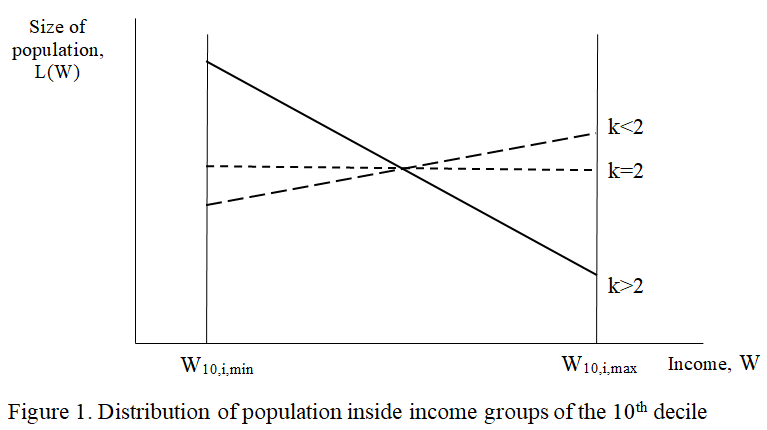
Table 4
Initial date on the incomes of the high–come groups of population, 2016
|
Decile groups and subgroups |
Size of subgroups, people |
Lower boundary of the annual income, RUB |
Higher boundary of the annual income, RUB |
Income of the group |
Average annual income of the taxpayer, RUB |
|
First |
11 493 000 |
0* |
102 230* |
1 053 993 998 400 |
91 707 |
|
Ninth |
11 493 000 |
529 533* |
728 471* |
9 038 135 064 000 |
786 403 |
|
Tenth |
11 493 000 |
728 471** |
– |
16 427 896 094 400 |
1 429 383 |
|
10.1 |
11 008 820 |
728 471 |
3 000 000 |
9 090 246 885 680 |
825 724 |
|
10.2 |
448 800 |
3 000 000 |
10 000 000 |
1 637 055 302 221 |
3 647 628 |
|
10.3 |
34 369 |
10 000 000 |
500 000 000 |
4 918 177 769 408 |
143 099 240 |
|
10.4 |
587 |
500 000 000 |
1 000 000 000 |
303 620 689 655 |
517 241 379 |
|
10.5 |
424 |
1 000 000 000 |
– |
478 795 447 436 |
1 129 234 546 |
*data for the whole population.
**data used both for the whole population and for the taxpayer.
As a result of the presented correction calculations, it is possible to form initial data necessary and sufficient for the assessment of the feasibility of introducing the PPIT (Table 4).
Expert risk assessment of the tax reform scenarios
The main risk of all tax reform scenarios is that the planned budgetary revenue will not be accumulated, consequently, the incomes of the high–income groups of population will not be duly reduced and, thus, the projected reduction of social inequality also will not happen. Keeping this in mind, the authors suggest a procedure of expert poll aimed at clarifying the feasibility degree of each of the four scenarios of the PIT reform. They compiled a questionnaire with just one question and methodological commentary for the surveyed experts: “Currently there are three scenarios of reforming the income tax system in Russian public discourse, presented by three political parties and based on the introduction of a progressive scale of taxation. Besides, there is an alternative scenario proposed by the Government, based on keeping the flat scale of the income tax with an insignificant increase of the tax rate (from 13 to 15%). Please give your expert opinion of the degree of feasibility of each of the four reform scenarios, taking into consideration that the increase of the tax rate will provoke tax evasion (last column of the Table). Your assessment should be on the scale from 0 to 100%, where 0 means that the consolidated budget will receive no additional revenue, and 100 means that the budget will receive the whole planned additional revenue”.
To simplify the assessment, the experts were given the table with a brief description of the four PIT reform scenarios: averaged assessments of the poll with the additional statistical characteristics are presented in Table 5.
The poll was of experimental character and included only 15 Russian economy experts specializing in the issues of taxation and knowledgeable about the taxation risks. The experts included representatives from Ural Federal University named after first president of RF B. Yeltsin (URFU), Southern Federal University (SFU), Financial University under the Government of the Russian Federation (FU), the Central Economics and Mathematics Institute of the Russian Academy of Sciences (CEMI).
The analysis of Table 2 shows that, according to absolutely all experts, the most reliable is the PIT reform scenario suggested by the Government of the RF, while the most unrealistic and unachievable one is a rather radical project of the LDPR. Compared to it, the CPRF project is more realistic, while the PJR project is even more feasible. The coefficient of polarization, understood as the difference between the maximum and the minimum assessments of the experts, showed that the smallest discord of opinions characterized the GRF project, and the greatest – that of the PJR. A low concordance for the PJR scenario is explained by the fact that it, being revolutionary in the sense that it proposes a transition from the flat to the progressive scale of the PIT, at the same time uses very modest quantitative assessments and has all the features of a palliative medium scenario which cannot lead to any noticeable social changes. Such internal contradictions affected the experts’ opinions and provoked a great diversity of opinions.
The obtained assessments of Table 5 are very important for understanding the true scale of the problem of tax reforms. For example, the tax collection in the GRF and the LDPR projects differs almost 12 times, which shows how hard it is to ensure an efficient transition from the flat to the progressive scale of the PIT. Such figures unequivocally prove that the establishment of a new ITNP scale will most likely be accompanied by a sharp drop in tax collection.
Table 5
Parameters of the four personal income tax reform scenarios in Russia
|
Scenario |
Annual income interval, RUB |
Tax rate |
Feasibility degree of the scenario, (D), in % (from 0 to 100) |
Range of assessments |
Polarization coefficient |
|
|
Lower boundary |
Upper boundary |
|||||
|
CPRF |
0 |
100 000 |
5% |
28.3 |
10–40 |
30 |
|
100 001 |
3 000 000 |
5000 RUB + 13% from the sum over |
||||
|
3 000 001 |
10 000 000 |
382 000 RUB + 18% from the sum over |
||||
|
10 000 001 |
– |
1 642 000 RUB + 25% from the sum over |
||||
|
LDPR |
0 |
180 000 |
0% |
8.3 |
0–20 |
20 |
|
180 001 |
2 400 000 |
13% from the sum over |
||||
|
2 400 001 |
100 000 000 |
288.6 th. RUB + 30% from the sum over |
||||
|
100 000 001 |
– |
29568.6 th. RUB + 70% from the sum over |
||||
|
PJR |
0 |
24 000 000 |
13% |
51.7 |
15–80 |
65 |
|
24 000 001 |
– |
3 120 th. RUB + 18% from the sum over |
||||
|
GRF |
Rate increase from 13 to 15% |
All categories of population except the poorest groups |
98.4 |
95–100 |
5 |
|
It should be noted that there is practically not alternative to the expert poll in the assessment of project risks. It is connected with the absence of any reliable statistical data on the feasibility of projected scenarios. No model constructions can give an opportunity to asses project risks based on the available statistical data. Meanwhile, the questionnaire survey procedure makes it possible to use the experience and intuition of experts, who in many cases very accurately predict the results of future reforms. If the experts are extremely carefully selected and their number is maximized (for example, to 100–150 people), it is possible to achieve a sufficiently high accuracy of assessment. If necessary, it is possible to use the procedure of open group discussion of the questionnaire and to obtain on its basis a series of group assessments, each of which will be based on consensus.
Results of analytical calculations
We have presented the preparatory analysis of different scenarios of tax reforms regarding the PIT, and below we are going to do analytical calculations with the purpose of obtaining practically relevant results. To achieve this, we will use the convolution of criteria (9) and obtain the integral evaluation of the scenario based on two parameters – the social and the fiscal one. To calculate the mass coefficient ζ , we are going to use the reasonable assumption that the fiscal and the social effects of the examined four scenarios in Table 5 are equal in sum. Then the condition for the calculation of the mass coefficient will look as following:
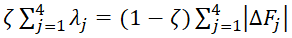 (13)
(13)
where j – the index of the tax reform project (four projects in total).
The calculations give the mass coefficient ζ=0.153. Then the integral criterion (9) for the evaluation of each project will look as following:
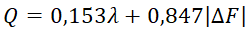 (14)
(14)
The calculations based on equation (14) make it possible to give a single fiscal–social characteristic of the analyzed scenarios (Table 6).
Table 6
Social and fiscal result of the PIT reform
|
Scenario of calculations |
Social inequality |
Revenues of the state |
||
|
Assets ratio (F) |
Change of the assets ratio (∆F) |
Absolute increment (∆T), trillion RUB |
Relative increment (λ), % |
|
|
CPRF |
13.7 |
–1.9 |
0.49 |
7.0 |
|
LDPR |
12.4 |
–3.2 |
1.02 |
14.5 |
|
PJR |
15.3 |
–0.3 |
0.27 |
3.8 |
|
GRF |
15.6 |
0.0 |
1.08 |
15.4 |
The assessments of the feasibility degrees for the tax reform projects obtained in the previous section make it possible to calculate the cumulative effect (11): E=QD. In this case, the index D is calculated as a share (D<1) and, as has already been mentioned, acts as a kind of efficiency coefficient. The results of applied calculations are presented in Table 7.
Table 7
Generalized assessment of the PIT reform scenarios
|
Reform scenario |
Integral criterion (Q) |
Feasibility degree (D) |
Generalized assessment (E) |
|
CPRF |
2.68 |
0.283 |
0.76 |
|
LDPR |
4.93 |
0.083 |
0.41 |
|
PJR |
0.83 |
0.517 |
0.43 |
|
GRF |
2.36 |
0.984 |
2.32 |
The obtained evaluations make it possible to range the projects on the PIT reform by the value of the expected actual (real) fiscal–social effect E. In particular, there are interesting shifts between the GRF, CPRF and LDPR projects. The four projects had the following rating by integral criterion Q: LDPR – 1, CPRF – 2, GRF – 3, PJR – 4. By the generalized assessment criterion, however, the hierarchy of projects looks completely different: LDPR – 4, CPRF – 2, GRF – 1, PJR – 3. Thus, the LDPR project, which was the most preferable one by its potential effect, moved into the last place when the risk of non-collection of taxes was taken into account, while the project of the GRF, on the contrary, rose from the third to the first place. At the same time, the PJR project slightly improved its position and moved from the last to the third place, while the CPRF kept its second place.
It is necessary to pay attention to the fact that the hierarchy of priorities established earlier [34] and based on a simple qualitative risk assessment of the PIT reform projects was exactly the same as the hierarchy based on the quantitative procedure that used the experts’ evaluations. It is another proof of the correctness and relevance of the obtained results. It means, in fact, that the qualitative assessment of the reform projects’ risks carried out by the authors matched the quantitative assessment obtained after surveying different experts. Obviously, this could be used in the future for the two-stage assessment of projects’ risks, when the first step consists of a rough qualitative assessment, which is specified, if necessary, at the second stage by a more precise quantitative evaluation.
These macroeconomic assessments make it possible to draw the following conclusions.
First, the results of introducing a progressive PIT scale are much more modest than it was declared in the analytical notes of the political parties. For example, the additional revenue from the reforms, according to the CPRF, should be 1.15 trillion rubles [10], while our assessment shows that it is 2.3 times smaller. It should be noted that the initial data for our calculations and those carried out by the CPRF were practically fully identical, so the results are comparable without any special reservations. This fact testifies to the existence of serious methodological drawbacks in the simplified macroeconomic calculations of the CPRF analysts. The assessment of additional revenue in the LDPR project was 2.05 trillion rubles [11], which also twice exceeds our assessment. And, finally, the 0.20 trillion rubles [12] from PJR are, on the contrary, 35% smaller than the final assessment of the authors.
Second, the above–mentioned overestimation of additional revenue from the tax reform makes it possible to conclude that a thorough adjustment of the initial data carried out in the previous section of this article is of great importance because without it the final figures may be greatly distorted. The main source of the emerging aberrations is that the analysts had a flawed understanding of the distribution of population inside income groups. Thus, the analytical materials of three parties were based on a simple averaging of the income relative to the boundaries of the income group and it was thus assumed that almost all taxpayers are either concentrated in the middle of the income interval or are evenly distributed inside it. Most likely, there is, in fact, a different pattern – most of the income group representatives have incomes close to the left boundary of the income interval. This distribution with a concentration in the left part is rather natural: the higher the income, the fewer people have it. This pattern is true not only for the intergroup distribution, but also inside the groups, including the high income subgroups. This fact should be taken into account in all the subsequent macro-calculations of the fiscal effects.
Third, the “soft” options of the progressive PIT scale are of no macroeconomic interest. Thus, for the PJR project the income disparity reduction effect is microscopic and will be imperceptible in real life; the increase of state revenue will be less than 4% from the current level of the PIT collection, which will have practically no effect on the size and stability of the country’s budget. Taking into account the transformational expenses for changing the flat PIT system and the high transactional expenses of the tax system in the future, we can quite confidently claim that this variant of tax reform is pointless. The efforts needed for the readjustment of the tax system will look hollow in view of the presented modest economic results. The LDPR project looks more radical and interesting, compared with “Just Russia” projects it results in a 10 times greater social effect in terms of reducing disparity and increases tax collection almost 4 times. The CPRF project is interim and too cautious to be viewed as a variant of serious reform.
Four, the fiscal potential of reforming the flat scale by increasing the rate from 13 to 15% is much higher than the potential of the progressive scale. This scenario results in more gains in tax revenue than the LDPR project, and certainly the other two projects. Thus, a minimal transformation of the tax system with the preservation of a flat scale can exceed the fiscal results predicted within even the most radical scenario of manipulating the progressive scale. This circumstance casts serious doubts regarding the feasibility of a large–scale PIT reform and transition to a progressive scale. The weakness of increasing the flat scale’s rate is its neutrality related to social inequality, which does not change in this scenario.
Fifth, the analyzed shifts in the rating system of the tax reform’s projects convincingly show that the risk factor is a significant element of the decision making system and can radically change the regulator’s preferences. Moreover, the volatility of the risk factor is much higher than the volatility of the fiscal-social effect. Calculations show that the maximum gap in the integral effect (Q) between the LDPR and the PJR projects was almost 6 times, while a similar gap in the feasibility criterion (D) between the PJR and the GRF projects reached 12 times. Thus, the differences between projects are mostly connected with the group of risk factors rather than the potential of tax revenues or the reduction of income disparity.
Conclusion
The analytical approaches to the evaluation of tax reforms presented in the article are a first step in the development of applied instruments of assessing reform projects. In this case, we took into account the social effect as the assets ratio, but in the general case the introduction of a progressive scale could affect not only the tenth, but also other decile groups, thus in more general calculations it is necessary to switch to the assessment of the social effect though the Gini index.
Besides, we examined the “volley” one–step reforms, while, according to modern requirements, a serious reform should be multi–step [35]. This means that the introduction of the PPIT should be extended over about 10 years and each 2–3 years certain elements of the new system should be introduced, thus avoiding any radical social shocks. For such an “extended” reform, it makes sense to evaluate the cumulative, i.e., summary effects for the 10 years of transformation.
However, the generalization of the analytical calculations scheme while taking into account the widening of the social groups affected by the reform and the reform period still does not disrupt the three–parameter scheme of reform projects which will be successful in this case as well.
Calculations presented in this article showed that the PIT reform scenarios are designed in such a way that they do not lead to any serious fiscal or social gains in the short term. It would be wrong, however, to conclude that the introduction of the PPIT is not feasible. It is beyond doubt that Russia with its class of super-rich people, should introduce a reasonable PPIT system. At present, however, there are two key conditions for this: the availability of adequate and timely information on the incomes of all citizens and a balanced PIT reform project. The first condition is absent now, but the rapid digitization of tax accounting gives hope for radical improvements of income statistics in the nearest future. The second condition is also absent, besides, there is no fruitful cooperation between political parties that support the introduction of the PPIT and the expert community that could develop such a reform project. The fate of the PIT reform depends on how successfully Russia overcomes these two obstacles.
References
1. Tanzi V. Fiscal Policies in Economies in Transition. Washington, D.C.: International Monetary Fund; 1992.
2. Burgess S. Taxation and Development. Journal of Economic Literature, 1993, vol. 31, no. 2, pp.797–801.
3. Cheasty A., Davis J. Fiscal Transition in Countries of the Former Soviet Union: An Interim Assessment. Economic Policy in Transitional Economies, 1996, vol. 6, pp.7–34.
4. Dabrowski M., Tomczynska M. Tax Reforms in Transition Economies – a Mixed Record and Complex Future Agenda. Series: Studies and Analyses, CASE, Warsaw, 2001. P. 36.
5. Hagemann R.P., Jones B.R., Montador B.R. Tax Reform in OECD Countries: Economic Rationale and Consequences. OECD Economics Department Working Papers, 1987, no. 40.
6. Agell J., Englund P., Sodersten J. Tax Reform of the Century – The Swedish Experiment. National Tax Journal, 1996, vol.49, no. 4, pp.643–664.
7. Lodin S.O. The Swedish tax system and inverted imputation. European Taxation; 1996. P.166.
8. Sinelnikov–Murylev S., Batkibekov S., Kadochnikov P., Nekipelov D. Assessment of results of reform of income tax in the Russian Federation. Moscow: Scientific works of IEPP; 2003. P. 120. (In Russ.).
9. Allingam M.G., Sandmo A. Income Tax Evasion: A Theoretical Analysis. Journal of Public Economics, 1972, no. 1, pp. 323–328.
10. Srinivasan T.N. Tax Evasion: A Model. Journal of Public Economics, 1973, no. 2, pp.339–346.
11. Yitzhaki S. A Note on Income Tax Evasion: A Theoretical Analysis. Journal of Public Economics, 1974, no. 3, pp. 201–202.
12. Lebedev V.V., Lebedev K.V. On the Application of the Verhulst Equation for the Analysis of Monetary Incomes Differentiation in Russia. Economics and Management: problems and solutions, 2017, no. 6, vol. 3(66), pp. 218–223. (In Russ.).
13. Grechanyi S.A., Rodin V.A. Rainbow Ratio and Possibility of Introducing a Progressive Tax in Russia. Proceedings of Voronezh State University. Economics and management, 2008, no. 2, pp. 44–47. (In Russ.).
14. Mirrlees J.A. An Exploration in the Theory of Optimum Income Taxation. Review of Economic Studies, 1971, no.38, pp. 175–208.
15. Saez E. Using Elasticities to Derive Optimal Income Tax Rates. Review of Economics Studies, 2001, vol. 68, pp. 205–229.
16. Smirnov R.O. Modeling of Choosing the Parameters of the Income Tax Schedule. St Petersburg University Journal of Economic Studies, 2011, no. 4, pp. 141–148. (In Russ.).
17. Davnis V.V., Rodin V.A. Modeling of the Progressive Taxation in Regions of Russia. Modern Economics: problems and solutions, 2016, no. 3(75), pp. 8–19. (In Russ.).
18. Ternovskii V.A. Mathematical Models of Taxation, Taking into Account Social Orientation. PhD (Econ.). Thesis. Voronezh; 2012. Pp. 16. (In Russ.).
19. Tishchenko A.S. Study of Income Tax Impact on the Structure of Population Expenses based on Modeling. PhD (Econ.). Thesis. Moscow; 2008. Pp. 20. (In Russ.).
20. Ashmarina U.V. Taxation of Personal Income in Russia: Prospects for Reform and Assessment of Fiscal Effects. PhD (Econ.). Volgograd; 2016. Pp. 163. (In Russ.).
21. Pickhardt M., Seibold G. Income Tax Evasion Dynamics: Evidence from an Agent–based Econophysics Model. CAWM discussion paper, 2011, no. 53, pp. 1–24.
22. Hashimzade N., Myles G., Page F., Rablen M. The Use of Agent–Based Modelling to Investigate Tax Compliance. TARC Discussion Paper: 004–13, 2013, pp. 1–29.
23. Flory J., Stöwhase S. MIKMOD–ESt: A Static Microsimulation Model of Personal Income Taxation in Germany. International Journal of Microsimulation, 2012, no. 5(2), pp. 66–73.
24. Fanti L., Manfredi P. Progressive Income Taxation and Economic Cycles: a Multiplier–Accelerator Model. Discussion Papers del Dipartimento di Scienze Economiche – Università di Pisa, 2003, no. 11, pp. 1–23.
25. Vinokurova T.P. Tax Risk: Economic Essence, Methods of Analysis and Assessment, Directions of Their Improvement. Economics and Management, 2012, no. 4, pp. 103–110. (In Russ.).
26. Laskina L.Y., Vlasova M.S. Tax Risk as an Integral Part of Business Risk. Scientific journal NRU ITMO. Series “Economics and Environmental Management”, 2015, no. 1, pp. 121–130. (In Russ.).
27. Egorova O.Y., Smirnova E.E. Tax Risk Management in a Company in Conditions of Economic Instability. Available at: https://nauchforum.ru/archive/MNF_social/2(21).pdf. (In Russ.).
28. Gordeeva O.V. Tax Risks: Concept and Classification. Finance, 2011, no. 1, pp. 33–36. (In Russ.).
29. Elgood T., Paroissien I., Quimby L. Tax Risk Management. Available at: https://www.pwc.com/gx/en/tax-management-strategy/pdf/tax-risk-management-guide.pdf.
30. Macijauskas L., Maditinos I.D. Looking for Synergy with Momentum in Main Asset Classes. European Research Studies Journal, 2014, no. 17(3), p. 3–16.
31. Polemis M. Panel Data Estimation Techniques and Mark Up Ratios. European Research Studies Journal, 2014, no. 17(1), p. 69–84.
32. Lykova L.N. A return to progressive personal income tax in the Russian Federation: some estimations. Journal of Tax Reform, 2018, vol. 4, no. 2, pp. 174–187. DOI: 10.15826/jtr.2018.4.2.051.
33. Mayburov I.A., Kireenko A.P. Tax reforms and elections in modern Russia. Journal of Tax Reform, 2018, vol. 4, no. 1, pp. 73–94. DOI: 10.15826/jtr.2018.4.1.046.
34. Balatsky E., Ekimova N. Comparative Characteristics of Progressive and Flat Income Tax Scales. Journal of Institutional Studies, 2018, vol. 10, no. 3. pp. 102–122.
35. Polterovich V. Elements of reform theory. Moscow: Ekonomika; 2007. P. 446. (in Russ.).
[1] In the existing system of flat taxation α=13%.
[2] See: Social position and living standard of population – 2017 г., Table 6.3.
[3] Ibid.
[4] See: Social position and living standard of population – 2017 г., Table 6.3.
[5] Ibid.
[6] См.: https://studfiles.net/preview/5316597/page:4/.
[7] См.: http://sozd.parlament.gov.ru/bill/427315–7.
[8] В соответствии с методикой Всемирной лаборатории неравенства примем за взрослое население людей, старше 20 лет.
[9] The re–calculation carried out for the adult population.
[10] See: http://sozd.parlament.gov.ru/bill/427315–7.
[11] See: http://sozd.parlament.gov.ru/bill/1148107–6.
[12] See: http://sozd.parlament.gov.ru/bill/384276–7.
Official link to the article:
Balatsky E.V., Ekimova N.A. Evaluating Scenarios of a Personal Income Tax Reform in Russia// «Journal of Tax Reform», vol.5, no.1, 2019, pp.6–22.