In the opinion of most businessmen and economists, one of the most important factors inhibiting production growth in Russia is its irrational fiscal policy that has been conducted virtually throughout the 1990s. The tax burden imposed by the state is believed to have been clearly excessive, not allowing enterprises to engage in normal economic activities. This fiscal pressure led to a whole series of negative phenomena. In the first place, business activity was constrained. Second, many capital–intensive industries that have priority from the standpoint of national interests were automatically cut off from profitable business spheres, initiating their gradual stagnation; as a result, the Russian economy underwent a structural degradation. Third, as it stimulated tax evasion and the development of a shadow economy, the unbearable tax pressure aggravated the country’s budget problems.

Under the present conditions, it becomes essential to assess the efficiency of the current system of fiscal regulation and to find ways of its optimization. These tasks can be accomplished by a variety of approaches, including, in particular, a qualitative method. This method involves the harmonization and improvement of the entire tax legislation. First of all, it is imperative to reject the practice of charging taxes on wages (at present, the value–added tax is collected precisely in this fashion) and it is enough to destroy a fairly normal economic structure and to move over to a scheme in which taxes are paid as funds are added to the enterprise’s account.

However, this approach, aimed at restructuring the entire accounting system in order to alter the mechanism of tax collection, does not involve methods of macroanalysis. In contrast, the quantitative method for optimizing the tax system aims to determine the most rational tax rates within the framework of the current fiscal mechanism. It is clear that it involves the optimization of the values of both individual tax rates and the aggregate tax burden on both legal entities and individual persons. This method does not imply any drastic change in the current tax system and basically aims only to adjust quantitative fiscal parameters. It is clear that this approach to improving the system of state regulation implies the application of a wide range of micro– and macroeconomic methods and models.

The efficiency of fiscal policy can be assessed from various perspectives, namely, from the standpoints of an economic entity (the source of taxes) and the state (the recipient of taxes). From the perspective of legal entities and individuals, the assessment of state fiscal policy is of no scientific interest because the logic here is plain and primitive: the more taxes, the worse. When assessing fiscal policy from the standpoint of the state, two aspects of analysis are possible: assessing the efficiency of state fiscal policy influencing the production activity of the economic system and influencing the revenue side of the state budget. As a rule, these two assessments conflict with each other, and a fiscal policy that is efficient with respect to the second criterion can be entirely inefficient with respect to the first one. Furthermore, even within the framework of each of these criteria, a fiscal policy can have ambiguous results; i.e., the development of the processes under study shows points of inflection.

It is the nonlinear dependence of the production output and tax revenues on the tax burden that is the subject of study when the efficiency of a fiscal system is assessed. As a rule, all specific calculations of efficiency parameters are based on A. Laffer’s curve, according to which the functional relationship between the state’s tax revenues and the level of tax burden is described by a parabola with a maximum point.

It should be acknowledged that the concept of Laffer’s curve occupies a central place in the modem theory of fiscal regulation. Specific investigations in this field usually proceed along two lines. The first (theoretical) line of research involves the economic modeling of production and fiscal processes and a theoretical derivation of Laffer’s parabolic dependence from the models thus constructed. In such studies, the emphasis is placed on providing rigorous proof of the presence of an inflection effect on the fiscal curve and determining its sources; this is of major importance for economic theory. Some of the most profound works along this line of research are [1–4]. The second (applied) line involves practical calculations of the values of Laffer points (points of inflections on the fiscal curve) for individual countries; this is in fact a special part of the theory of macroeconomic assessment. In this case, the functional features of the economic system take second place to computational algorithms and work on specific statistical data (see, e.g., [5–8]). In some cases, theoretical models are accompanied by empirical calculations, thereby merging the first and second approaches. However, such investigations are extremely limited in number, and this approach–although quite attractive–appears to be inefficient.

Within each of these two lines of research, there are different approaches to the problem. They can be divided into three broad groups. The first group of studies is characterized by the microeconimic approach to describing the system [1, 3–5]. The results obtained for an individual entity are extrapolated to all economic agents, thereby attuning the necessary degree of generality in the analysis. The second group uses essentially aggregated model£ [2, 7, 8], making it possible to perform macrogeneralizations and to ignore the internal structure of the economy. Attempts to combine the two approaches have usually proved inefficient.

Let us examine more closely some possible approaches to assessing the efficiency of state fiscal policy and check the more efficient of them on the basis of Russian data for 1990–1998.

Formulation of the Problem and Method of Study

In recent years, there have been many investigations attempting to assess the efficiency of individual aspects of the fiscal system by finding Laffer points for specific types of taxes. The studies [1–8] examined the following taxes: value–added, profit, wages, property, income, and other taxes. At the same time, the idea of Laffer’s curve was from the start conceived to fit the concept of the aggregate tax burden, i.e., the entire mass of taxes collected. In the discussion that follows, we shall adhere to this understanding of the problem and, hence, Laffer points will be sought for the averaged macroeconomic index of the tax burden. This index is here defined as the gross domestic product (GDP) share of tax revenues in the country’s consolidated budget (in a more general case, it is possible to use the gross national product).

This study is based on the assumption that the production output X, reflected by the GDP value, depends on the level of tax burden θ = T/X, where T is the sum of tax revenues in the country’s budget. The dependence X(θ) is approximated by a nonlinear function whose parameters can be quantitatively estimated. The identification of the X(θ) function will enable Laffer points to be calculated. We will distinguish Laffer points of the first and second kind (a similar approach was used in [6]). Here are the relevant definitions.

A Laffer point of the first kind is a point θ* at which the production curve X = X(θ) reaches a local maximum, i.e., when the following conditions are met: dX(θ*)/dθ = 0 and d²X(θ*)/dθ² < 0. A Laffer point of the second kind is a point θ** at which the fiscal curve T = T(θ) reaches a local maximum, i.e., when the following conditions are met: dT(θ**)/dθ = 0 and d²T(θ**)/dθ² < 0. Economically, a Laffer point of the first kind signifies the tax burden limit at which the production system does not go into recession. A Laffer point of the second kind shows the tax burden value beyond which an increase in the mass of tax revenues becomes impossible.

By identifying two Laffer points and comparing them with the actual tax burden, it is possible to assess the efficiency of the country’s tax burden and its optimization paths. Let us examine some approaches to this problem.

Econometric (statistical) methods for assessing the efficiency of fiscal policy

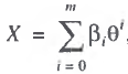
In the general case, this problem can be solved by econometric methods, on the assumption that the production output depends nonlinearly on the tax burden value. In this case, it is sufficient to approximate the GDP value by a polynomial regression of the form:

                                                                                                      (1)

where β_i, denotes parameters to be assessed statistically on the basis of retrospective dynamic series.

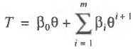
Taking into account formula (1) and the tax mass:

                                                                                        (2)

we can write the following relation:

                                 (3)

To perform the relevant calculations, the entire data set should be represented by the dynamic series of the two “primary” parameters, X and T. Knowing these quantities, one can calculate by Eq. (2) the retrospective series for the secondary parameter θ. Subsequently, in the course of computational experiments, polynomial (1) of corresponding degree is found. It is desirable that this should be a quadratic or, at least, cubic function, because a higher order of the polynomial will subsequently make it more difficult to find Laffer points (polynomials     of degree three and higher lead to the multiplication of stationary points of the production curve X = X(θ) and require an additional procedure for their filtering in order to identify Laffer points among them).

Considering the specific character of smoothing operations, econometric models of type (1) have a number of obvious peculiarities. First, in order to obtain β_i, values, one must have sufficiently lengthy and statistically adequate dynamic series. Second, the β_i, parameters are constant in time, leading in some cases to the invariability of Laffer points (in particular, this situation exists for a quadratic function). This is not quite justified, because it would be more logical to assume that Laffer points are time–variable quantities.

It should be noted that the approach proposed above, which is based on a primitive polynomial approximation of economic growth by tax function (1), is intended to solve a purely technical, instrumental problem without regard for intrasystem economic relations. The functional properties of the system are not explicitly modeled, but they are indirectly reflected in dependence (1). Although functional dependence (1) is nonlinear, regression (1) is linear with respect to its parameters and, hence, there are no particular technical difficulties encountered in its identification. This is one of the substantial advantages of the model scheme proposed here.

Analytical (algebraic) methods for assessing the efficiency of fiscal policy

Considering that retrospective dynamic series that would be sufficient for specific econometric calculations are not yet available for the Russian economy, one can resort to other methods for assessing the efficiency of fiscal policy. Among such alternative approaches are methods of piecewise pointwise approximation of the process by a power function; these methods are fundamentally different from econometric methods, which are based on interval approximation. In this case, for each basic point representing a given period (in our case, a year), one constructs its own function X = X(θ) with corresponding values of its parameters. Considering that there can be more than one parameter in the function, their unambiguous estimation requires additional information on the increments of the variables in time. Considering the nonlinear relationship between the production output and the level of tax burden, the approximating function should be a quadratic polynomial. Two calculation options are possible here: a generalized three–parameter option and a simplified two–parameter option. Let us examine them in greater detail.

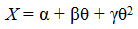
1. Three–parameter method. This method is based on the approximation of economic growth by a three–parameter quadratic function, in which the argument is the level of tax burden:

                                                                                           (4)

where α, β, and γ are the parameters to be estimated.

Then, according to (2), the sum of tax revenues is given by

                                                                  (5)

At each point in time, the GDP value depends on the level of tax burden, and the character of this dependence is defined by (4). However, relation (4) is insufficient to unambiguously determine the three parameters α, β, and γ; therefore, it is necessary to set up another two equations that would include these parameters. Such equations can be written by passing from functions (4) and (5) to their differentials:

                                                                 (6)

      (7)

When passing from relations (4) and (5) to (6) and (7), we used the assumption that the differentials of the variables X and θ are satisfactorily approximated by finite differences: dX ~ ΔХ; dT ~ ΔT, dθ ~ Δθ. This assumption is traditional in computational mathematics, and appears quite legitimate for the case under discussion. Then, in applied calculations, the indices ΔХ, ΔT, and Δθ denote the increments of the corresponding quantities during one time interval (year) between two basic points; i.e., ΔX_t = X_t+1 – X_t; ΔT_t = T_t+1 – T_t; and Δθ_t = θ_{t +1} – θ_t, where t is the index of time (year).

Thus, Eq. (4) describes pointwise economic growth, i.e., at a specific time t, whereas Eqs. (6) and (7) portray the “interval” growth of the production output and tax revenues during the period between the current (t) and succeeding (t + 1) basic points. According to this approach, Eqs. (4) and (5) define families of production and fiscal curves, whereas relations (6) and (7) portray their curvature, thereby enabling the sought functional dependencies to be selected from these families.

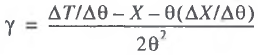
This computational scheme is based on the composition of the system of equations (4), (6), and (7) and its solution with respect to the parameters α, β, and γ, allowing this scheme to be described as analytical or algebraic. The solution of the system (4), (6), and (7) yields the following formulas for the parameters to be estimated:

                                 (8)

                                                            (9)

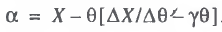                                                                                (10)

By identifying the parameters of functions (4) and (5), it is easy to determine Laffer points. A Laffer point of the first kind θ*, when dX/dθ = 0, is determined from the formula

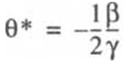                                                                                                  (11)

and a Laffer point of the second kind θ**, when d²T/dθ² = 0, is found by solving the following quadratic equation:

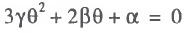                                                       (12)

and is ultimately calculated by the formula

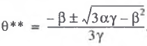                                                                                   (13)

An additional investigation of the properties of functions (4) and (5) will make it possible to determine whether the stationary points obtained are Laffer points. If the stationary points are points of a local minimum or their values fall outside the tolerance range [0; 1], then, Laffer points are absent.

An alternative to this three–parameter method is the approach based on the use of a truncated third–degree polynomial as the production function: X = αθ + βθ² + γθ³. The number of parameters remains unchanged, being still three. In this case, the procedure for finding Laffer points is adjusted for the initial cubic dependence, and stationary points for the fiscal curve will be found by solving a cubic equation. It is clear that this algorithm can generate two Laffer points of the second kind. In my opinion, owing to its lower ambiguity and greater convenience, the first, basic variant of the three–parameter method should be used in practice.

It should be noted that the analytical (algebraic) method for assessing the efficiency of fiscal policy makes it possible to use functional dependencies with not more than three, parameters. A greater number of parameters makes it necessary to supplement the basic system (4), (6), and (7) by additional equations, but this is impossible owing to the narrow formulation of the initial problem.

2. Two–parameter method. This method is based on the approximation of economic growth by a truncated quadratic function including only two parameters:

                                                                       (14)

Then, the sum of tax revenues is equal to

                                                                                                 (15)

An additional restriction imposed on the functional properties of the production system is defined by the following equation, which is similar to (6):

                                                                                         (16)

The system of equations (14) and (16) is sufficient for finding the parameters β and γ. As in the case of the three–parameter method, Eq. (14) portrays the pointwise properties of the production system, whereas Eq. (16) portrays the interval properties. The auxiliary equation defining the dynamic properties of the fiscal system is absent; by default, it is assumed that the amount of taxes is entirely determined by the activity of the production system and the level of fiscal pressure.

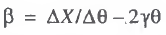
The formulas for estimating the parameters on the basis of (14) and (16) are as follows:

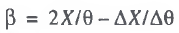                                                          (17)

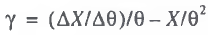                                                  (18)

Laffer points of the first and second order are determined from (14) and (15) according to the corresponding formulas:

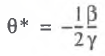                                                                                                        (19)

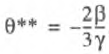                                                                                                       (20)

Analysis of the second–order conditions shows the following: in order for the stationary points (19) and (20) to be Laffer points, it is necessary and sufficient that the following two inequalities be satisfied: β > 0 and γ< 0.

Comparative study of methods for assessing the efficiency of fiscal policy

Within the class of algebraic methods, two approaches to calculating the efficiency of the fiscal system by means of Laffer points are possible. Let us analyze the specific features of each in order to select the most acceptable approach for further calculations.

Let us begin with the econometric approach. As noted above, the order of the polynomial regression should not be too high because as it increases, the economic meaning of the smoothing procedure is lost. The fact is that, in the limiting case, when the order of polynomial (1) is equal to  – 1, where  is the number of basic retrospective points (years), the number of parameters to be estimated will likewise be equal to . In this situation, it is pointless to use statistical methods for constructing the regression, because all parameters can be unambiguously determined algebraically by interpolating the initial dynamic series of X by polynomial (1). Thus, in the limiting case, statistical methods pass into algebraic, illustrating their original methodological unity. However, the interpolation procedure should, generally speaking, be avoided for a number of reasons.

First, high–degree polynomials require a high accuracy of calculations because, otherwise, statistical errors are accumulated. Second, polynomials of degrees higher than four generate serious algebraic problems during the subsequent determination of stationary points. In this case, the problem reduces to solving an algebraic equation of degree five or higher, which in itself is very complicated. However, even after this problem is solved, all stationary points should be classified into local minima and maxima, after which Laffer points should be selected out of points of local maxima. In addition to the aforementioned problems, one will ultimately have to interpret the results obtained, yet another difficult task. Third, the very procedure of a priori interpolation implies that there is a rigorous functional relationship between the output and the level of tax burden. Although there must be a theoretical relationship between these two variables, it is still desirable that its presence should be strictly proven. Furthermore, even though polynomial interpretation is technically faultless, it appears somewhat artificial in terms of meaning.

The construction of a regression dependence is also fraught with many disadvantages. To begin with, Russia still lacks a data set for forming dynamic series that would yield efficient regression models. Second, the Russian economy of the transition period showed no stability in the development of the process under study. For example, during some years, an increase in the tax burden was accompanied by a decrease in the GDP, whereas, during other years, by its rise. In fact, this means that some hypothetical functional relationship between the GDP and tax burden is constantly disrupted, with each short period characterized by its own production function; an attempt to find a universal dependence for the entire period under study is unlikely to be successful. It is this fact that dictates the use of two– and three–parameter analytical methods for esti­mating Laffer points as the simplest methods that most adequately correspond to the present economic conditions.

The use of parametric methods is based on the premise that there is a functional relationship between production output and tax burden. The form of this relationship is common to all years analyzed, but its parameters vary. These parameters are estimated according to a sliding scheme, i.e., separately for each pair of years. The first year is the base year, and the second year plays an auxiliary role when determining the production–function parameters of the first year. This approach appears to be the most promising for the next five or six years until data on stabilized economic growth are accumulated.

A comparison of the two algebraic methods proposed leads to the following conclusions. The main advantage of the three–parameter method is that it takes into account the functional properties of both production function (4) and fiscal function (5). Consequently, the estimated parameters are simultaneously constrained by the properties of the production and fiscal systems, which can be substantially different in practice. The two-parameter method is confined to the properties of the production curve (14) alone; this signifies an undoubted simplification of the process modeled and leads to more crude estimates. Furthermore, the form of the initial quadratic production function (4) is more general than formula (14), thereby yielding a richer analytical scheme. In this sense, the three–parameter method is preferable. At the same time, the computational simplicity, convenience, and elegance of the end results of the two–parameter calculation scheme predetermines its choice as the working procedure. It appears that, in order to understand the macroeconomic situation, one should use the simplest algorithms that do not lead to ambiguous interpretations.

Analysis of the properties of the production and fiscal systems

Elaborating on the last thesis, I will show that the two–parameter scheme for finding Laffer points is the most acceptable from a theoretical point of view. To prove this, it is sufficient to analyze the properties of the production and fiscal curves.

If Laffer points of the first and second kind for dependencies (14) and (15) exist, then, the production curve and its analogue in the form of the fiscal curve will appear as shown in the figure. It is not difficult to see that the production output and tax revenues synchronously go to zero at two points: θ = 0 and θ = –β/γ. Thus, the active regions defining the production and fiscal functions coincide. It is readily apparent that if –β/γ = 1, the ultimate level of tax burden at which the production and fiscal systems completely collapse is equal to 100%. At 0 < –β/γ < 1, the production and fiscal collapse begins earlier; in the case of –β/γ > 1, both systems continue to function even after the complete withdrawal of profits from economic entities. The values of the production output and taxes collected at the 100% level of fiscal burden in all cases coincide, corresponding to the theoretical assumption, and are equal to Х(1) = T(1) = β + γ.

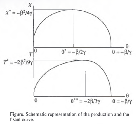
However, the most important and interesting inference that can be drawn is the Laffer points of the first and second kind do not coincide, with the Laffer point of the second kind being shifted to the right along the tax axis relative to the point of the first kind: θ**>θ* (this follows directly from formulas (19) and (20) and can be visualized by geometrically superimposing the production and fiscal curves depicted in the figure). Thus, the production and fiscal curves are characterized by different curvatures. One might say that the fiscal curve can be obtained by the deformation of the production curve toward its right–hand margin. The maximum production output X* coinciding with a Laffer point of the first kind is X* = –β²/4γ; the maximum mass of tax revenues T* coinciding with a Laffer point of the second kind is T* = –2β²/9γ.

This regularity in the mutual arrangement of Laffer points of the first and second kind appears to be very important. This is because modern tax theory deals mainly with Laffer points of the second kind, without giving due attention to Laffer points of the first kind. At the same time, as I see it, a constructive analysis of the fiscal system should involve three parameters: θ, θ*, and θ**. The fact is that in some cases the situation when θ* < θ < θ** can appear. It means that the actual tax burden is lower than the Laffer point of the second kind and, hence, from the standpoint of the state’s financial interests, has a fairly normal value. However, it is higher than the Laffer point of the first kind, and this means that the existing tax pressure stimulates a decline in production, thereby conflicting with this country’s long–term economic interests.

The foregoing leads to the conclusion that, ideally, the fiscal system should be adjusted to meet the condition θ* > θ, because the tax pressure must not undermine the economic activity of enterprises.

The theoretical scheme of the production and fiscal systems depicted in the figure appears to be perfectly simple and logical. At the same time, it clarifies some points of tax theory that had not been quite clear. This is the decisive factor in selecting the two–parameter method as the most suitable technique for the practical assessment of the efficiency of fiscal policy under the conditions of the Russian economy.

Database for analytical calculations

The initial information for our calculations consisted of statistical data on tax revenues and GDP presented in [9–11]; an additional source of information was [12]. However, some indices appearing in these data sets are incompatible. For example, the revenue structure of the consolidated budget has changed since 1995. In particular, the “Nontax Revenues” section had the “Other Revenues” heading until the end of 1994 [9], which was later removed. In order to level off the dynamic series for “Tax Revenues” and to obtain comparable data for 1990–1998, we summed the data under the headings “Sum of Taxes” and “Other Revenues” for 1990–1994. The series thus corrected is presented in Table 1. Although this approach is not irreproachable, its use in aggregate calculations is quite permissible; for more subtle calculations, the initial information should be polished more carefully.

Table 1. GDP and tax revenues of Russia’s consolidated budget in 1990–1998 (in trillion rubles)

An important consideration in subsequent calculations is that all of the methods for estimating Laffer points described above work for macroindices calculated in both current and comparable prices. Even in theoretical studies, both current and deflated tax revenues are examined separately [7]; depending on this, the differential properties of the fiscal curve vary widely. In fact, this is a separate important problem of tax theory, because the effects for current and deflated tax revenues differ strongly owing to the powerful influence from inflationary tendencies.

In view of this, the subsequent calculations will be performed according to two scenarios: for tax revenues in current (scenario 1) and comparable (scenario 2) prices. The year 1990 is taken as the reference point. Note that the two–parameter computational scheme for estimating Laffer points is invariant with respect to the data on the GDP and tax revenues and, therefore, handles both scenarios in an identical manner.

Computation results

The results of calculations by formulas (17)–(20) for the initial data given in Table 1 according to scenarios 1 and 2 are presented in Tables 2 and 3.

Analysis of Tables 1 and 2 leads to some interesting conclusions, outlining the evolution of fiscal relations in Russia.

Table 2. Calculated fiscal parameters of the Russian economy in 1990–1998 (scenario 1)

Table 3. Calculated fiscal parameters of the Russian economy in 1990–1998 (scenario 2)

I. Throughout the period analyzed, the fiscal system of the Russian economy underwent constant disturbances, of which there were at least two manifestations.

First, there was a significant spread in the values of the actual tax burden: from 21.5% in 1996 to 27.4% in 1993; this difference amounts to 27% of the 1996 base and is fairly perceptible for any economy. Second, there was no single trend in the dynamics of the actual tax burden, which constantly displayed up and down fluctuations. This disoriented economic agents and predetermined contradictory results of all subsequent calculations, which only reflected the overall uncertainty in the country’s economic situation.

II. The data in Table 2 relating to scenario 1 indicate that not all of the years analyzed show the presence of Laffer points. For example, out of eight years, it was only in the years 1990, 1993–1995, and 1997 that Laffer points of both kinds within the tolerance range were detected; in the remaining years, the detected stationary points were points of local minima, and hence, they do not fall under the definition of Laffer points. From a geometrical point of view, this means that the fiscal and production macroeconomic curves are constantly arched either upward (producing local maxima) or downward (forming local minima). This effect is yet another indication of the extreme instability of the fiscal processes.

III. Comparing the fiscal points θ, θ*, and θ** derived from calculations according to scenario 1, one may argue that almost throughout the transition period, the level of actual tax burden in Russia covered both Laffer points. This means the following: the country’s tax system was constructed in such a way that it stimulated a decline in production with a simultaneous reduction in the state tax revenues. Any increase in the fiscal pressure only served to further exacerbate the situation in the real sector. A slight improvement came only in 1997, which was one of the most favorable years throughout the period of economic reform. The situation that year was highly unusual: the level of the actual tax burden θ was higher than the Laffer point of the first kind θ* and lower than the Laffer point of the second kind θ**. This median position of the θ parameter signifies the following: in 1997, the tax burden was set sufficiently high to inhibit economic growth, yet at a fairly acceptable level so as not to cause a further collapse of the budget. In other words, at that time, the fiscal interests of the state came into conflict with the purpose of maintaining a long-term economic growth, with the fiscal component of macroeconomic policy prevailing. In order to switch the economic system from recession into growth, it was necessary to decrease the tax burden by only 3%, but, as a result, the revenue side of the consolidated budget would have suffered.

IV. The identification of Laffer points according to scenario 2 showed that these points existed only in 1991, 1992, 1995, and 1996. In 1991, the actual tax burden occupied an intermediate position between the points θ* and θ**, very closely approaching θ** (the gap between them was as little as 0.3%). In 1992, the “fiscal resistivity” of the Russian economy increased, but the new shifts in the tax system led to a significant rise in the tax burden, exceeding even the limit set by the Laffer point of the second kind. Thus, the state again acted to the detriment of its own fiscal interests, let alone the interests of Russian producers. Such careless actions by the government in the tax sphere are reflected in clearly degenerate results for 1993–1994: the Laffer points assumed negative values. Geometrically, this means that, throughout the tolerance range, the production and fiscal curve behaved monotonically; from an economic point of view, this is equivalent to a situation in which economic agents respond unidirectionally to any tax changes. Such periods are characterized by general “fiscal indifference,” which testifies to serious problems in state regulation. However, the aforementioned fiscal depression was immediately followed in 1995 by a dramatic improvement of the tax climate: for the first time, the actual tax burden was below both Laffer points. It was in that period that the premises for economic growth were created. In the next year, the situation slightly deteriorated: the actual tax burden was once again between the two Laffer points. The following year, 1997, was another year of fiscal indifference, neutralizing all preceding positive shifts.

V. On the whole, calculations according to scenario 2 confirm the conclusions drawn from the scenario 1 quantitative estimates: the actual tax burden in the transition–period Russian economy was excessive; insignificant fiscal indulgences during some of the years did not change the general pessimistic picture.

Methodological and economic comments

The quantitative results obtained and their analysis have outlined some points that require a special discussion. Let us examine the most important of them.

To begin with, calculations according to both scenarios demonstrate an extreme instability of Laffer points, which serve as the principal indicators of the efficiency of state fiscal policy. In view of this, it would be legitimate to ask: How such jumps are to be understood? Furthermore, in addition to the fiscal factor, there are many equally significant aspects of economic life that are neglected in the methods proposed here. Moreover, under certain circumstances, the fiscal regulator can be of secondary importance as compared to them. Is it then possible to ignore the other aspects of economic growth?

As I see it, these questions do not reject the methodology developed above. On the contrary, given that each period is marked by new disturbances in the system, the dependence X = X(θ) itself is reorganized, as reflected in the adaptive procedure for recalculating its parameters. Owing to constantly renewing parameters, we can determine the role and significance of the fiscal factor. Occasionally, fiscal instruments lose their relevance and the production dynamics begins to be governed by some other variables. Such times are characterized by fiscal indifference, and any rearrangement of various groups and factors and their effects on economic growth can cause strong fluctuations of Laffer points.

Second, calculations according to the two scenarios yield rather inconsistent results. For example, the years marked by the absence of Laffer points according to scenario 1 (1991, 1992, and 1996) exhibit these points according to scenario 2. Or the unsuccessful (according to scenario 2) year 1997 turns out to be quite satisfactory according to scenario 1. These facts prompt some serious questions. For instance, are these discrepancies a consequence of the methodological incorrectness of the method used? If not, then which scenario should be preferred?

These questions compel a reconsideration of some points of tax theory. In my view, there are no serious contradictions in the results, given that scenario 1 takes into account the response to a change in the tax burden from both the production output and the average level of prices, whereas scenario 2 takes into account the effect of production adjusted for inflation. In view of this, the more optimistic results obtained according to scenario 1 should be treated with great caution, and scenario 2 should be given preference when analyzing fiscal effects. Therefore, scenario 1 can be used mainly as auxiliary in analytical investigations.

Third, the following important question remained outside the analysis: When detecting an overly high level of tax burden, which specific taxes should be reduced? Or it is necessary to resort to proportionate, across–the–board reduction of all taxes?

Unfortunately, there is no single answer to these questions. Across–the–board tax reduction should be considered irrational, because it means a large–scale disturbance of the tax system, which nearly always has negative effects. In such cases, the focus should be on sales tax, value added tax, property tax, and income tax. It is these fiscal instruments that are the most efficient and the least detrimental to economic entities. On the whole, decisions of this kind must be made with due regard for taxing practice rather than theory. Nevertheless, the estimates of the possible reduction of the tax burden can provide a useful clue when making the final decision. In addition, the two–parameter method used here can be applied to specific taxes. For example, it is fairly easy to construct dynamic series for the value added and the relevant tax and to establish a relationship between them by the algorithm described above. It is quite realistic to construct similar series for population incomes and tax revenues from income tax; for the property of individual persons and property tax, etc. Such detailed calculations will provide clues to a rational fiscal policy by indicating which taxes should be raised and which should be reduced.

Thus, the proposed scheme for assessing the efficiency of fiscal policy by calculating Laffer points involves a further development and modification of the underlying idea, attesting to its practical validity and fruitfulness.

Concluding the discussion concerning the efficiency of the fiscal policy of the Russian state, I would like to touch upon some important points related to its assessment.

In the first place, one of the advantages of parametric methods is their descriptive character. In my previous work [6], I propounded the subjectivity of all quantitative estimates obtained with optimization schemes and models; this drawback does not apply to parametric methods. In fact, the entire class of algebraic methods passively reproduces the functional properties of the production system in the fashion of a black box without any a priori postulates and premises. This fact makes parametric methods theoretically and methodologically neutral, and hence, most objective.

Second, constructing dynamic series of estimates of the efficiency of fiscal policy (Laffer points) is of major importance for forecasting the results of the state fiscal policy. At the present stage, however, confidence in such forecasts is undermined by the extraordinary instability of all economic processes; more or less reliable forecasts are only possible in the presence of persistent production–fiscal trends. In my view, a practical criterion for determining whether or not this requirement is met is the stability of Laffer points over a period of at least three to five years (fluctuations between their extreme values should not exceed 2–3%). So far, this criterion is unrealistic. In view of this, although the tax burden in the Russian economy has been excessive during the last decade, one cannot claim without serious reservations that its decrease will lead to an automatic increase in production activity. However, unless the years to come bring economic cataclysms, the probability of this outcome is fairly high.

Third, in addition to other things, a retrospective assessment of Laffer points performs an indicative function. For example, the discovery of a situation in which the actual tax burden is shifted to the right beyond both Laffer points can signal the appearance of serious clashes between the interests of producers and the state. However, in order to raise the efficiency of the indicative function of such calculations, it is necessary to collect reliable information more promptly. At present, the entire budgetary statistics operates with great delay, preventing any timely monitoring of the current situation.

Fourth, my study has provided yet another confirmation of the conclusion that there is no single method for assessing the efficiency of fiscal policy by means of Laffer points. Even within the bounds of algebraic methods, it is possible to use both two– and three– parameter computation procedures. This fact alone testifies not so much to the need for new methods as to the need for comparative analysis of the available methods in order to select the main method that should dominate analytical investigations. In my opinion, this should be the principal target of further efforts to improve the tools for assessing the efficiency of fiscal policy.

References

1. Sokolovskii, L.E., Podokhodnyi nalog i ekonomicheskoe povedenie (Income Tax and Economic Bahvior), Ekon. Mat. Met., 1989, vol. 25, issue 4.

2. Movshovich, S.M. and Sokolovskii, L.E., Vypusk, nalogi i krivaya Laffera (Issue, Taxes, and Laffer’s Curve), Ekon. Mat. Med., 1994, vol. 30, issue 3.

3. Arkin, V., Slastnikov, A., and Shevtsova, E., Nalogovoe stimulirovanie investitsionnykh proektov v rossiiskoi ekonomike (Tax Incentives for Investment Projects in Russia’s Economy), Moscow: RPEI; Fond Evraziya, 1999.

4. Kapitonenko, V.V., Inflyatsionnyi sdvig nalogovoi stavki na krivoi Laffera, Ekon. i tekhnol.: mezhvuz. sb. nauch. tr. (Economics and Technology: An Intercollegiate Collection of Scientific Papers), Moscow: REA, 1994.

5. Gusakov, S.V. and Zhak, S.V., Optimal’nye ravnovesnye tseny i tochka Laffera (Optimal Equilibrium Prices and the Laffer Point), Ekon. Mat. Med., 1995, vol. 31, issue 4.

6. Balatskii, E.V., Lafferovy effekty i finansovye kriterii ekonomicheskoi deyatel’nosti (Laffer’s Effects and Financial Criteria of Economic Activity), Mirovaya ekon. i mezhdunar. otnosheniya, 1997, no. 11.

7. Balatskii, E.V., Tochki Laffera i ikh kolichestvennaya otsenka (Laffer Points and Their Quantitative Estimation), Mirovaya ekon. i mezhdunar. otnosheniya, 1997, no. 12.

8. Balatskii, E.V., Nalog na imushchestvo firm i nakoplenie osnovnogo kapitala (Corporate Property Tax and Fixed Assets Accumulation), Mirovaya ekon. i mezhdunar. otnosheniya, 1999, no. 3.

9. Finansy v Rossii. Stat. sb (Finances in Russia: A Statistical Collection), Moscow: Goskomstat Rossii, 1997.

10. Rossiiskii statisticheskii ezhegodnik. Stat. sb. (Russian Statistical Yearbook: A Statistical Collection), Moscow: Goskomstat Rossii, 1997.

11. Rossiiskii statisticheskii ezhegodnik. Stat. sb. (Russian Statistical Yearbook: A Statistical Collection), Moscow: Goskomstat Rossii, 1998.

12. Sotsial’ no–ekonomicheskoe polozhenie Rossii. 1998 god. Spr (Social and Economic Position of Russia 1998: A Handbook), Moscow: Goskomstat Rossii, 1999.

Official link to the article:

Balatskii E.V. Efficiency of State Fiscal Policy// «Studies on Russian Economic Development», Vol.11, No.5, 2000, pp. 439–447.