
Many concepts and effects figure in economic science today, and they are fundamentally significant for the functioning of economic systems. In this article we give a systematic exposition of two phenomena that are not well–known in the Russian literature: Wagner’s law and the Armey–Rahn curve, as well as the paradox of wealth, which is connected with them.
Wagner’s law: Its general formulation, significance, and consequences
Wagner’s law has figured in economic theory for a fairly long time as one of the most unshakeable economic laws. It was formulated by the German economist Adolph Wagner in 1892. Various adaptations of this law can be found today, but many of them are completely incorrect. In its current interpretation, in our opinion, this law should be formulated as follows: growth in gross domestic product (national income) is accompanied by accelerated growth in government spending.
This assertion can be easily formalized. If X is gross domestic product (GDP) and G is the amount of government spending, then according to Wagner’s law the following exponential function takes place:
 (1)
(1)
where m and θ are parameters, with m>0 and θ>1.
Thus, Wagner’s law postulates an increasing, nonlinear relationship between government spending and GDP. If θ≤1, then Wagner’s law is automatically violated. In other words, in the language of mathematics, Wagner’s law is equivalent to the assertion that in relationship (1) the parameter θ is strictly greater than one: θ>1 (Figure 1).
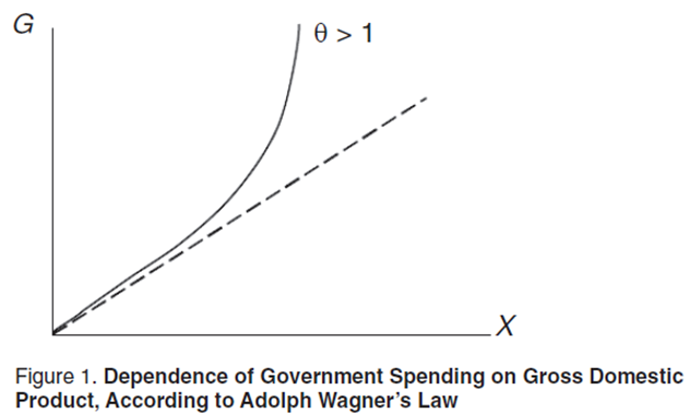
If we look at the GDP elasticity of government spending, it coincides with the parameter θ, that is, θ=(X/G)(dG/dX). In this case, Wagner’s law asserts that the elasticity of government spending with respect to GDP is greater than 1. Consequently, Wager’s law postulates that economic growth acts as an accelerator of growth in government spending. Because of this, some researchers interpret this law as a particular case of the ratchet effect [1]. Henceforth we will call the exponential function in Figure 1 the Wagner curve.
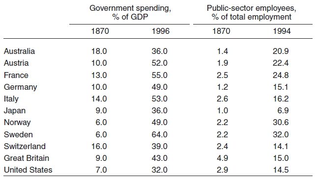
Substantively, Wagner’s law means that over the course of time the role of government increases and, along with it, the scale of the public sector. And it is necessary to state that this thesis has been fulfilled with uncommon constancy for a long time. In Table 1 it is easy to see that for more than 120 years there has been consistent growth trend in government revenues as a percentage of GDP, which is a direct consequence of Wagner’s law.
Table 1. Parameters of Government Spending and the Public Sector in Leading World Countries.
It is perfectly obvious that sooner or later Wagner’s law has to be violated because its limit is 100 percent confiscation of company earnings and their subsequent distribution through the budget. However, such socialization of finances is equivalent to eliminating the private sector as such, which is impossible by definition. Thus, in spite of how unshakable it is in retrospect, by no means can Wagner’s law be considered a truly universal relationship. In some sense, it is only a question of when this law will cease to be in effect. This is the reason that many economists have recently shown interest in Wagner’s law. However, despite its apparent simplicity, verifying this law involves certain methodological nuances, which basically explains the existing differences of opinion as to whether Wagner’s law is being fulfilled or violated.
Verification of Wagner’s law: Long–run elasticity
Based on previous constructions, we can say that, in practice, verifying whether Wagner’s law is being fulfilled or violated amounts to econometric estimation of the elasticity parameter θ. To do this, analysts construct an econometric relationship based on which the elasticity θ is then computed.
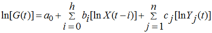
An econometric model of the following type is generally used for such a purpose [2]:
 (2)
(2)
where a0, bi, and cj are parameters of the model that can be statistically estimated; t is the time index (year); and Yj is the jth factor influencing the dynamics of government spending. We will explain relationship (2).
First, the model includes the relationship between government spending and GDP distributed in time (X(t – i)). Experience shows that the amount of lag can be as much as five years. With this approach, the effect of economic growth on budget policy can be taken into account more precisely and completely.
Second, in addition to the GDP factor, the model includes other factors (Yj) on which budget policy depends. There are three or four such “other” factors. This approach makes it possible to filter out the effect of GDP on government spending from other perturbations. In some studies, other factors are also used with a time lag. In the simplest case, just one other factor may be used, for example, the amount of government spending in previous periods. Sometimes a trend component is added to the right side of model (2) [3].
Third, the model takes logarithms of all the original variables. This is done to make it more convenient to compute the elasticity θ later.
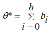
We should dwell on the last point in somewhat greater detail. The fact is that the “complete” GDP elasticity of elasticity is made up of “partial” elasticities taking into account the time step. Thus, the lag relationships lead not to a point elasticity θ, but to a distributed elasticity θ*, which is called long–run elasticity in the literature because it takes into account remote (past) changes in GDP that have influenced the amount of government spending in the present. In connection with this, the form of equation (2) proves to be extremely convenient for computing long–run elasticity:
 (3)
(3)
From equation (3) we can see that the long–run elasticity of government spending with respect to GDP is the simple sum of the regression coefficients preceding all of the GDP figures, taking the time lag into account. On the whole, the parameter θ* is an empirical estimate of the theoretical parameter θ, and henceforth they can be used as synonymous concepts.
In applied studies, the verification of Wagner’s law is reduced to a two–step procedure: constructing model (2) and computing the value of (3). As in theory, when θ*>1, Wagner’s law is fulfilled, otherwise it is considered violated. The study of this dichotomy is the basic topic of economists’ discussion regarding Wagner’s law in the contemporary world.
In our opinion, it is impossible not to note that Wagner’s law is essentially empirical, rather than economic. In other words, it cannot be derived from any general theoretical considerations. This effect is not established as a universal component in either the logic of economic development or the psychology of economic agents. Accordingly, the verification of Wagner’s law today is done purely empirically, which dictates econometric tools for estimating elasticity θ.
Discussion regarding Wagner’s law: A new regime for international economic development
Despite the agreement that exists in the scientific world about how to verify Wagner’s law, its empirical verification does not prove to be easy and it is the source of much discussion. Some researchers believe that Wagner’s law has not yet lost its significance and continues to operate, while others think that its time has passed because it is violated in most cases.
For example, in 2008 Serena Lamartina of the European Central Bank and Andrea Zaghini of the Bank of Italy published their calculations in relation to Wagner’s law [4]. Their study shows a quite mixed picture. For instance, they used two estimation procedures, which generated completely different results. According to one procedure, beginning in 1997, the group long–run elasticity of government spending with respect to GDP for economically developed (Organization for Economic Cooperation and Development; OECD) countries was less than 1 – (θ* < 1) – which indicates violation of Wagner’s law. However, calculations using the other model, which is more precise in the opinion of the Italian economists, indicate that in all these years this elasticity was significantly greater than 1 – (θ* > 1). Thus, the final verdict depends largely on the estimation procedure that is selected.
However, even if we accept the hypothesis about the operation of Wagner’s law to which Lamartina and Zaghini subscribe, there is an obvious inhomogeneity in the group of countries the authors studied. In some countries the elasticity is much lower than 1, while in others it is clearly greater than 1. Consequently, there is good reason to maintain at least the following: the countries of the world are gradually being divided into two groups: relatively poor countries, where Wagner’s law is still in effect, and relatively wealthy countries where it no longer operates.
In 2010, Dick Durevall of the University of Gothenburg (Sweden) and Magnus Henrekson of the Research Institute of Industrial Economics (Sweden) published an article in which they quite categorically rejected the hypothesis that Wagner’s law is still relevant [5]. According to their calculations, Wagner’s law operated throughout the period from the 1860s until the end of the 1960s in Sweden, and from the 1860s until the end of the 1970s in Great Britain. However, after that the law lost its force and is not in effect today. The Swedish economists also noted a pronounced asymmetry effect in the British economy, according to which government spending grows faster in bad years and much more slowly in good ones. On the whole, Durevall and Henrekson are inclined to conclude that Wagner’s law has a limited sphere of action, and in the long run it is violated.
Based on the above, we can conclude that in developed countries Wagner’s law began to lose its significance in the 1980s. At present, the trend is continuing and encompassing more and more new countries.
It makes sense to say a few words here about pitfalls in the process of verifying Wagner’s law. The point is that various combinations of model data are used in applied calculations. For example, sometimes just the aggregate of government spending is used on the left side of (2), and sometimes its increment. In some cases, GDP in current prices is used on the right side of model (2), but in other cases GDP in constant prices is used. Sometimes absolute GDP appears in the right side of (2), and sometimes per capita GDP. Of course, all of these cases can create diverse combinations, which in itself can produce qualitatively different results of the calculations.
As an example, we point out a modeling method that is used fairly often, in which the left side of (2) has the amount of government spending, and the right side has per capita GDP. However, the distorting effect of scale automatically occurs here. If the effect of population growth is removed by using per capita GDP, then the same should be done with budget spending, which should also be converted to a per capita figure. Otherwise, the effect of population growth (or decline) is taken into account in one statistical aggregate, but not in the other. With this approach, if the population is growing, the GDP elasticity of government spending is automatically overestimated, and if the population is declining, it is underestimated. If the elasticity is in the narrow zone around one, then such a shift of estimates could lead to fundamental distortion of the result, when, for example, violation of Wagner’s law is erroneously confirmed.
In an effort to bring clarity to the question of Wagner’s law, we will perform the simplest calculations for two countries: Sweden and Russia. In some sense, these two countries complement each other: Sweden is a classical capitalist country that went through the stage of constructing a strong public sector long ago, while Russia is a transition economy that is still in the stage of formation of a public sector.
The calculations that were done for Sweden for the period 1990–2007 enabled us to construct the following elementary econometric relationship [6]:
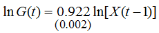 (4)
(4)
N=18; R²=0,999; DW=1,14; Е=0,7.
In model (4) we use the following notations: N is the number of observations; R2 is the coefficient of determination; DW is the Durbin–Watson statistic; and E is the mean error of approximation (in percent of the actual value). Values of the standard errors are indicated in parentheses under the regression coefficients. The model passed the basic statistical tests.
Analogous calculations for Russia for the period 1990–2007 enabled us to construct the following model:
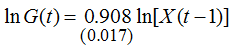 (5)
(5)
N=18; R²=0,994; DW=0,99; Е=12,3.
The constructed models (4) and (5) have good statistical characteristics, which means that they are quite highly reliable. Note that in both models the lag is only one year. This is apparently because the budget is generally set based on the past year’s spending, and more remote values of GDP already lie in the aggregates of previous years’ spending. Thus, the long–run elasticity of spending has a tendency to turn into ordinary short–run elasticity in recent time.
The main conclusion from models (4) and (5) is that the elasticity for Sweden and Russia is less than one: θ*=0.92<1 and θ*=0.91<1, respectively. At least two conclusions follow from this.
First, Sweden and Russia have had very similar regimes for establishing government spending depending on the amount of GDP. This fact can be partly explained by the similar social model in the two countries, which is based on a considerable role of the public sector in the economy.
Second, Wagner’s law is violated in both Sweden and Russia. Thus, we get additional confirmation of the verdict that this law is on its last legs. However, it seems that we are only at the beginning of this process, since the deviation of the elasticities from the critical line is still obviously insignificant. In this situation, a temporary reanimation of Wagner’s law is not out of the question if the economic trend deteriorates.
Thus, our calculations confirm that the international economy is in a state of transition: it is obviously deviating from Wagner’s law but has not nearly abandoned it yet.
The Armey–Rahn curve and the Scully point
We spoke above about the internal contradiction in Wagner’s law involving movement toward total state control of finances (we will arbitrarily call this phenomenon the “communism effect”). However, there is an effect in the economy that, being a natural limiter of Wagner’s law, works much sooner than the infamous communism effect. This effect is called the Armey–Rahn effect, which we will consider in greater detail.
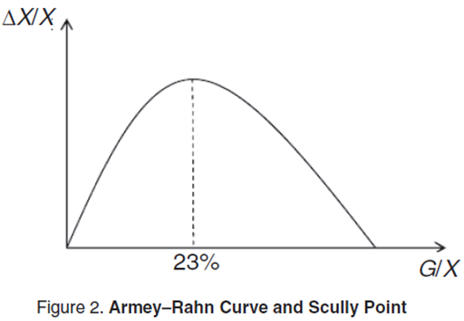
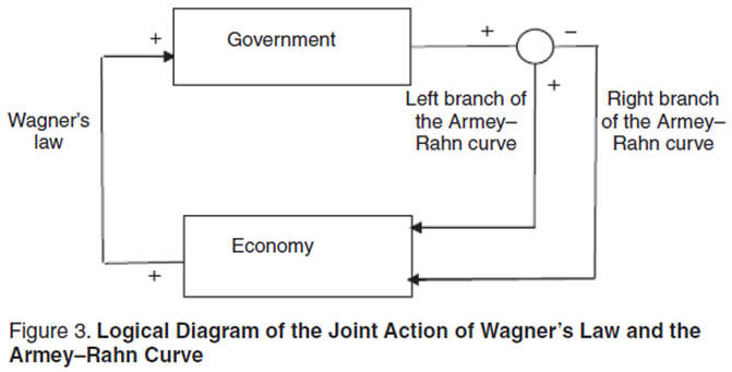
According to Wagner’s law, growth of GDP influences the growth of government spending, thereby establishing feedforward in economy/government subsystems. However, as it turns out, there is also feedback between these subsystems, which has enormous significance. If the scale of government is measured by the percentage of government spending in GDP (g=G/X), then the dependence of a country’s economic growth rate (ΔX/X) on the scale of government (g) has the form of a parabolic function, with the maximum point characteristic of it. In the economic literature, such a curve is sometimes called a Rahn curve, sometimes an Armey curve, and sometimes, in a more generalized way, an Armey–Rahn curve (Figure 2). Henceforth, we will use its generalized name, which it was given in honor of the economists Richard Armey and Richard Rahn, who popularized it and made this dependence a working tool of contemporary economic analysis [7].
It should be said that the parabolic form of the Armey–Rahn curve has a double meaning. First, as we said previously, it indicates the presence of an inverse effect of budget (government) activity on economic growth, and second, this relationship proves to be negative, that is, stabilizing. In other words, if, according to Wagner’s law, GDP growth accelerates growth in government spending, then, according to the Armey–Rahn curve, in a certain stage growth in the percentage of government spending in GDP leads to a slowdown in GDP growth. Thus the Armey–Rahn effect turns the economy/government system into a self-regulating market system in which development of events in one direction only is not permitted.
Meanwhile, the presence of a maximum point on the Armey–Rahn curve implies that the forces limiting the scale of the government’s participation go into operation only when some critical value of the parameter g has been reached. Up to that point, expansion of the public sector can occur quite harmlessly in the economy. A general view of a cybernetic diagram combining Wagner’s law and both parts of the Armey–Rahn curve is shown in Figure 3.
In the scientific community, there have been discussions for a long time about what level of government spending should be considered the maximum permissible. For instance, Gerald Scully, who studied the effect of budget policy on economic growth for many years, estimated the maximum point on the Armey–Rahn curve at 23 percent [8]. Henceforth, we will call this the Scully point (Figure 2), although we will immediately specify that this number should not be given too much significance, since there can be no talk about any standards here. Each country has its own conditions, which give rise to their own values of the Scully point. By analogy with the Laffer point, we can define the Scully point as the point for which the conditions ∂λ/∂g=0 and ∂2λ/∂g2<0 are fulfilled, where λ=ΔX/X and g=G/X.
At present, the Scully point seems to be clearly underestimated and beyond the possibilities of most national regulators. At the same time, we should not underestimate the effect of deviation from the Scully point. For example, Daniel Mitchell of the Heritage Foundation’s Thomas A. Roe Institute for Economic Policy Studies gave an extremely dramatic illustration of the power of the Armey–Rahn curve’s effect. In the United States, the share of government spending in GDP was 35.7 percent in 2003, as opposed to 47.6 percent in the EC–15. This almost 12 percent–point advantage, led to 40 percent higher per capita GDP in the United States in that year than in the EC–15 ($37,600 versus $26,600), and the average GDP growth rate for the period 1993–2003 was 50 percent higher (3.2 percent versus 2.1 percent) [9]. Thus, there are serious grounds for thinking that the stronger positions of the government in Europe makes it less dynamic and wealthy in comparison with the United States.
While constructing the Armey–Rahn curve presents certain difficulties, its presence makes it possible not only to understand how mistaken budget policy is but also to estimate the real economic losses that occur because of deviation to the right of the maximum point.
The Armey–Rahn curve: Empirical verification
In general, the Armey–Rahn curve can be approximated by various classes of functions, but the simplest and most natural seems to be a quadratic relationship that defines a parabola in coordinates G/X and ΔX/X, as in Figure 2.
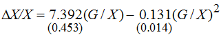
Econometric calculations for Sweden for the period 1990–2007 enabled us to construct the following model:
 (6)
(6)
N=18; R²=0,998; DW=0,88; Е=3,4.
Analogous calculations for Russia for the same period gave the following relationship:
 (7)
(7)
N=18; R²=0,995; DW=0,37; Е=5,7.
On the whole, both models have good statistical characteristics (other than the presence of autocorrelation of the remainders in model [7]), which makes it possible to use them in subsequent analytical calculations.
Based on the constructed models, we can draw several quite important conclusions.
First, the Armey–Rahn curve does exist and can be satisfactorily approximated by a parabolic function. So the given analytical construct is by no means a theoretical phantom but can be re–created based on the simplest statistical parameters. Moreover, the relationships proved to be identical for countries as dissimilar as Sweden and Russia, which suggests that the Armey–Rahn curve is invariant across various countries and that the macroeconomic correlation between the GDP growth and the percentage of government spending is stable.
Second, the Armey–Rahn effect actually does exist and gives rise to the Scully point as some maximum of possible economic growth. This fact directly follows from analysis of the signs of the parameters in models (6) and (7), as well as the form of the curves generated by them. In this case, the maximum points lie in the region of permissible values, which indicates the absence of degenerate cases.
Third, the values of the maximum points are obviously greater than the Scully point. For instance, for Sweden it is g*=38.7 percent, and for Russia g*=28.0 percent. In both cases, the maximum points lie quite far from the classical Scully point (23 percent). This fact indicates that traditional fears that growth in the share of budget spending in GDP could strongly inhibit economic growth are exaggerated. It seems that the economy’s limit of tolerance is still somewhat higher than is customarily thought. Even taking into account that the models we have constructed are fairly crude and might yield more modest estimates of g* with additional calibration, the figures obtained would still hardly come close to the classical Scully point.
The latter conclusion has great theoretical significance in that the Scully point is used for additional economic interpretations. For example, Lawrence Hunter of the Institute for Social Choice and Individual Values gives a graph in his work that shows the Armey–Rahn curve and the Laffer curve together [10]. In this case, the Laffer point is to the right of the Scully point, and this means that government spending policy has a stronger restraining impact on economic growth than does tax policy. Furthermore, some economists interpret the gap between the Laffer point and the Scully point as a zone of seeking pure rent. Our calculations confirm this position of the Laffer curve and the Armey–Rahn curve in relation to each other [11]. At the same time, we should make a small remark: Figure 4 shows the Laffer production curve and the Laffer point of the first kind corresponding to it. If we look at the fiscal curve and the Laffer point of the second kind corresponding to it, then they almost coincide with the Armey–Rahn curve and the Scully point.
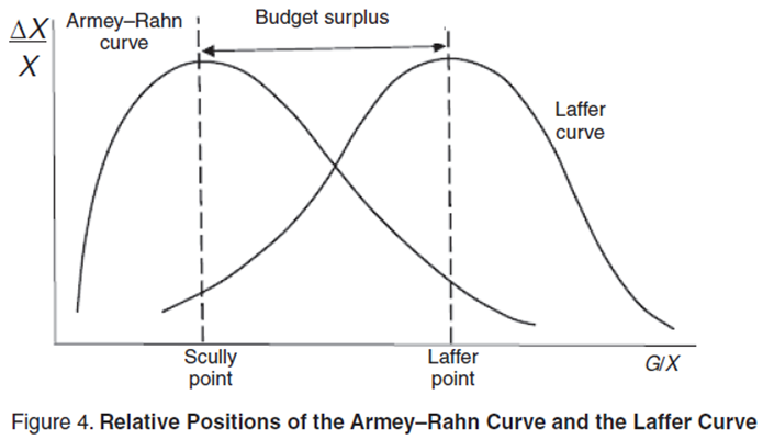
It should be noted that the position of the two curves in relation to each other in Figure 4 implies a somewhat idyllic fiscal policy consisting of strict collection of taxes at the level of the Laffer point, followed by their incomplete spending on government needs. This actually means that the government always has some budget surplus. However, sometimes, for example, for Russia, cases can occur in which the Laffer point of the first kind is greater than the Scully point. In this case, the difference between the two points can be interpreted as the maximum permissible budget deficit. On the whole, the scheme used previously by Hunter should be acknowledged as perfectly correct.
The paradox of wealth
Combining Wagner’s law and the Armey–Rahn curve in a single analytical construct produces an extremely interesting result, which we will call the paradox of wealth, which we examine in greater detail.
According to Wagner’s law, equation (1) takes place, in which θ>1. Then, taking (1) into account, the percentage of government spending in GDP (g=G/X) can be described by the following equation:
 (8)
(8)
On the strength of Wagner’s law, function (8) is increasing; however, this increase can be painless for the economy until it exceeds point g* (the Scully point), which exists in accordance with the requirement of the Armey–Rahn curve. When g>g*, production starts to decline. Then, equating the function (8) to the value of g*, we get the following equation for the limiting amount of GDP:
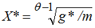 (9)
(9)
Equation (9) indicates the maximum amount of GDP, beyond which GDP itself can no longer grow. At this point, we arrive at the paradox: GDP growth limits its own growth. Of course, this paradox makes sense only if Wagner’s law is fulfilled, when θ>1. Thus, the joint action of Wagner’s law and the Armey–Rahn curve erects a barrier to growth of the national economy. We can only assume that upon reaching this barrier the economy will simply run in place, maintaining the level of wealth that has been attained.
It follows that Wagner’s law acts as a serious limit to the economy’s long–term growth. Accordingly, to eliminate the paradox of wealth it is necessary to neutralize Wagner’s law. Consequently, the need to violate Wagner’s law is part of economic evolution itself, with the economic growth that characterizes it. It is precisely in wealthy countries that have stepped over the barrier (9) that the economic development regime is restructured, with a change in the value of the elasticity of government spending from θ>1 to θ<1.
The paradox of wealth explains well the nature of displacement of Wagner’s law from the international economy: first it is violated in the wealthiest countries with high GDP, and some time later in poorer countries, which in turn reach the necessary level of production, and so on.
We have discussed various aspects of Wagner’s law above, but some confusion remains as to how strong it is and whether it can produce undesirable effects in the foreseeable future. To deal with this issue, it is necessary to probe the numerical patterns and clarify the order of the quantitative effects that occur. For this purpose, we believe it is quite sufficient to determine how quickly “communism” sets in if Wagner’s law is fulfilled. In this case, by communism we mean the point g=1, when all of the GDP that is created is confiscated in the form of taxes and then redistributed in the form of government spending.
Here we should specify that, just as Wagner’s law is not always fulfilled, the Armey–Rahn curve does not have an automatic effect. Cases can be presented when, for example, this curve will not have a maximum point. In this case, the effect of Wagner’s law will be unlimited, and the system will tend toward the infamous point of communism g=1. From relationship (8), it is easy to derive a function for growth in the percentage of government spending:
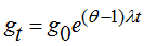 (10)
(10)
where λ is the GDP growth rate; and g0 is the percentage of government spending in GDP at the initial moment in time t.
From this it is easy to derive a relationship for estimating the period (T) in which the economic system reaches the state gT=0:
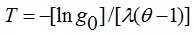 (11)
(11)
Using equation (11), we can perform the simplest scenario calculations, which are given in Table 2.
Table 2. Versions of Reaching the State g = 1.
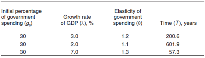
Wagner’s law turns out to be a very complex phenomenon. On the one hand, with a moderate acceleration coefficient (e.g., when θ=1.1) and “natural” economic growth (2 percent per year), it is not a serious threat, since it takes a whole epoch comparable with the lifetime of a civilization (600 years) to reach communism. On the other hand, with a high acceleration coefficient (e.g., when θ=1.3) against the background of prolonged economic overheating (7 percent), it harbors a danger of relatively quick collapse of the private sector, literally in two generations (50 years). Note that, according to available estimates, the elasticity in Greece is θ=1.40; and in Spain, θ=1.25 [12]. Consequently, a ratchet effect in the direction of Wagner’s law can be really significant and, as a result, destructive. Analogously, a 7 percent annual growth rate of the economy is not out of the question and has been typical, in particular, of China in recent decades, which once again indicates how realistic the dangerous scenario is.
Consequences of violation of Wagner’s law
We have shown above that in the past 150 years the international economy has undergone fundamental changes in the sense of reorganizing interaction between the public and private sectors. How are these changes manifested?
Fulfillment of Wagner’s law led not only to growth in the government’s financial strength but also to growth in the private sector of the economy in physical terms: number of employees, accumulated fixed assets, amount of investments and production, and so on. This means that over the course of many years the public sector has increased its share of the economy, suppressing the private sector, as it were. It can be said that a unidirectional effect of displacement of the private sector by the public sector has been at work in the economy. Accordingly, violation of Wagner’s law, with a corresponding deformation of the Wagner curve, has stopped this process. At present, a regime of interdependent development of the two sectors on the basis of competition has been established in advanced countries.
From the perspective of dynamic effects, the public sector’s share has ceased to increase monotonically and has changed over to a fluctuating mode. Moreover, the range of fluctuations shows a tendency to decrease with time. In metaphorical language, the interaction of the two sectors can be represented as an hourglass filled almost to the brim. Accordingly, the structural changes in the economy are similar to turning over this hourglass. But no matter how much you turn it, the original gap in its volume will not change, and the difference between the public and private sectors will not be too large. That is approximately what is happening now in the national economy: the volume of the two sectors pulses in search of the optimal relationship. The main result of such a change in regime is the formation of a so–called privatization cycle in the economy, which means fluctuation of the public sector’s share. Something similar is happening with the percentage of government spending in GDP: its dynamics has become extremely unstable and experiences constant sudden changes up or down [13]. Thus, in the national economy the dynamics of the percentage of government spending in GDP generally has reversing tendencies.
We should point out that the change in the international economy’s regime has made questions concerning the privatization cycle very timely: its presence or absence, its length, and its amplitude. In this case, the dynamics of the percentage of government spending in GDP loses its significance in comparison with the dynamics of the public sector’s share, for example, of employees. This is because the dynamics of the percentage of government spending in GDP is characterized by extreme instability and has a pronounced sawtooth trajectory, due to the problem of uneven replenishment and spending of budget resources as well as all kinds of distortions in estimating monetary aggregates. The dynamics of the public sector’s share, on the other hand, has a certain smoothness, reflecting fundamental shifts in the disposition of the two sectors that are taken into account in physical terms.
Thus, violation of Wagner’s law means the culmination of a long period of strengthening of the government’s position and the formation of a new type of economic cycle in various countries: a privatization cycle. In this case, it can already be stated that this cycle is gradually developing into small fluctuations. For instance, while periods of privatization and nationalization were easily seen in various countries in the past, now they have become less noticeable. In this regard it is sufficient to recall that even the international crisis of 2008, contrary to all expectations, did not lead to large–scale nationalization of the economy, not only in the United States, but even in Russia. Thus, the policy for managing the privatization cycle is gradually turning into a fine-tuning tool, indicating once again that Wagner’s law is on the way out.
Notes
1. D.Durevall and M.Henrekson, “The Futile Quest for a Grand Explanation of Long–Run Government Expenditure,” Research Institute of Industrial Economics, IFN Working Paper, no.818 (2010).
2. S.Lamartina and A.Zaghini, “Increasing Public Expenditures: Wagner’s Law in OECD Countries,” Universidad de Salamanca, 2008, http://campus.usal.es/~XVEEP/PAPERS/J1S6/XVEEP-29 percent20LAMARTINA-ZAGHINI.pdf.
3. Ibid.
4. Ibid.
5. See Durevall and Henrekson, “The Futile Quest for a Grand Explanation of Long–Run Government Expenditure.”
6. The author is deeply grateful to N.A.Ekimova for her help in collecting the data and doing the calculations.
7. See L.A.Hunter, “The Leviathan Project,” Institute for Social Choice and Individual Values, 2008, www.socialsecurityinstitute.com/uploads/File/The-Leviathan-Project-Web.pdf.
8. Ibid.
9. See D.Mitchell, “The Impact of Government Spending on Economic Growth,” Heritage Foundation, 2005, www.heritage.org/Research/Reports/2005/03/The-Impact-of-Government-Spending-on-Economic-Growth/.
10. See Hunter, “The Leviathan Project.”
11. See E.V.Balatskii [Balatsky], “Otsenka vliianiia nalogovykh instrumentov na ekonomicheskii rost,” Problemy prognozirovaniia, 2004, no.4.
12. Lamartina and Zaghini, “Increasing Public Expenditures.”
13. E.V.Balatskii [Balatsky] and N.A.Ekimova, “Tipologiia privatizatsionnykh tsiklov,” Obshchestvo i ekonomika, 2007, no. 9–10.
Translated by James E. Walker
Official link to the article:
Balatsky E.V. Wagner’s Law, the Armey–Rahn Curve, and the Paradox of Wealth// Problems of Economic Transition, vol. 54, no.12, 2012, pp. 40–54.